In this section, we are going to look at 2 important elements of a shiny app :
a reactive object.
a module.
We will also introduce briefly the package bslib, to give to the shiny app a more modern look.
54 Reactive object
This part presents what is a reactive object : how it works and why it is (so!) useful.
In the previous examples, we created 3 simple output elements : a table, a chart, a text.
To create those visuals, we proceeded the same way, in 4 steps :
Get data.
Filter data.
Transform data.
Create the result (a table, a chart, a text).
Very often, the first 3 steps are the same. Then instead of repeating those steps several times, we can simply create a reactive object, and then use it as an input to create the visuals.
By doing so we keep the code easier to maintain (less lines), and faster to update. Instead of updating the 3 steps of each objects, we simply need to update the ones of the reactive object.
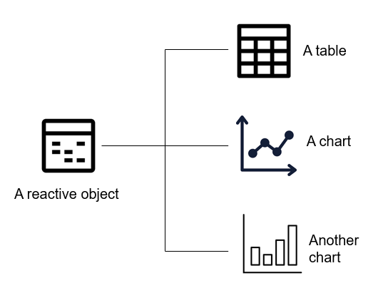
As described in the figure below, a reactive object is used as an input for a table and 2 charts.
Figure 86 : from a reactive object to charts
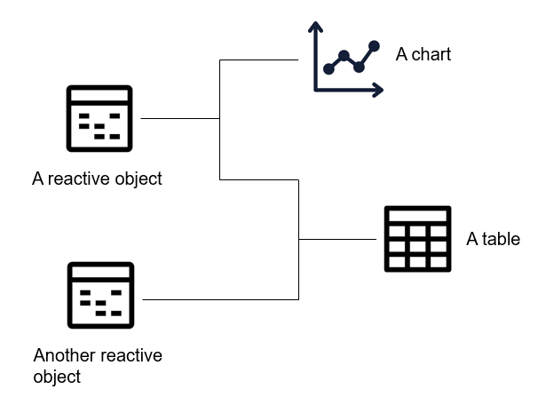
Furthermore, a reactive object can be combined with another one to create a visual, or another reactive object for instance.
This is very useful when we want :
to perform a calculation and then take its result (stored as a reactive object) to combine it with another set of data (another reactive object for example).
to use a “write back” capability :
the user inputs some data in the UI, and then those data can be used to update another table (in the server), to run some calculations or create some new visuals.
Figure 87 : combination of 2 reactive objects
Let’s illustrate how to create and use a reactive object, a data frame, continuing on the previous examples.
To create a reactive object, we need to write the following syntax : name_of_the_reactive_data <- reactive({ })
Within the 2 parentheses and curly bracket ({ }), we will :
proceed with the steps to import, filter and transform the data.
keep the final result, using the function return().
Then, to use this reactive data frame, we simply need to affect it to another object, within the 2 ({ }) of an output.
for example, to get some reactive data, we write : df1 <- name_of_the_reactive_data().
note : we must put 2 brackets after the name of the reactive object.
we can also make sure the object df1 is then a data frame, so we can add the syntax : df1 <- as.data.frame(df1) .
In the code below, we then notice that :
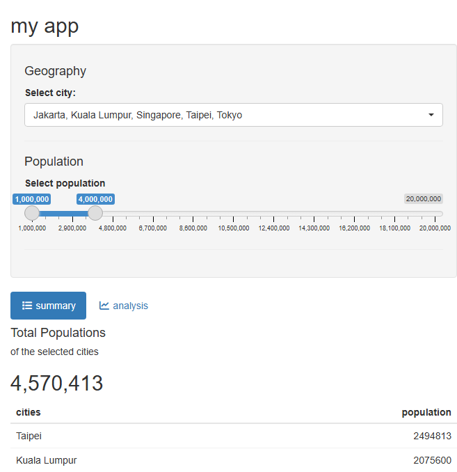
we start creating a reactive data frame, called react_selected_data.
this reactive object is then used to create to visuals : a table and a text.
We simplified the overall code : we just need to update the reactive object if we want to make some changes, for example adding a new filter or performing a transformation.
#----------------------# Upload libraries#----------------------# shinylibrary(shiny)library(shinyWidgets)# ETLlibrary(tidyverse)# tablelibrary(reactable)# chartslibrary(highcharter)#----------------------# Upload data or create datasets#----------------------cities <-c("Taipei", "Tokyo", "Singapore", "Kuala Lumpur", "Jakarta")population <-c(2494813, 14254039, 6110200, 2075600, 10684946)my_data <-data.frame(cities, population)#------------------------------------------------## Shiny app##------------------------------------------------#------------------------------------------------## SHINY UI##------------------------------------------------# Define UI ----ui <-fluidPage(# App title ----titlePanel("my app"),# Sidebar layout with input and output definitions ----sidebarLayout(# Sidebar panel for inputs ----sidebarPanel(conditionalPanel(condition ="input.tabselected == 1 || input.tabselected == 2",h4("Geography"),pickerInput("Selected.cities","Select city:",choices =sort(unique(my_data$cities),decreasing =FALSE),options =list(`actions-box`=TRUE,`live-search`=TRUE),multiple = T,selected =unique(my_data$cities)[1:1000]#selected = c("Taipei") # if we want a preselection ),hr() ), # close conditionalPanelconditionalPanel(condition ="input.tabselected == 1",h4("Population"),sliderInput( "Selected.population", "Select population", min =1000000, max =20000000, value =c(1000000, 4000000) ) ), # close conditionalPanelhr(),width =2 ), # end of SidebarPanel# Main panel for displaying outputs ----mainPanel(# Output: Tabset w/ plot, summary, and table ----tabsetPanel(type ="pills",tabPanel("summary", icon =icon("list"), value =1,fluidRow(column(3,h4("Total Populations"),h5("of the selected cities"),h2(textOutput("total_cities_populations_TX")) ),column(4,reactableOutput("summary_RT") ),column(5) ) # close fluidRow ),tabPanel("analysis", icon =icon("chart-line"), value =2,highchartOutput("cities_populations_HC") ),id ="tabselected" ), # close tabsetPanelwidth =10 ) # end of mainPanel ))#------------------------------------------------### SHINY SERVER###------------------------------------------------server <-function(input, output) {#------------------------------------------------# Create reactive#------------------------------------------------ react_selected_data <-reactive({#------------------# Get data df1 <- my_data#------------------# Filter# Select city df1 <- df1 |>filter(cities %in% input$Selected.cities)# Select population df1 <- df1 |>filter(population >= input$Selected.population[1] & population <= input$Selected.population[2])#------------------# Transform#------------------# keep resultsreturn(df1) })#------------------------------------------------# Table 1# Display of Summary table#------------------------------------------------ output$summary_RT <-renderReactable({#------------------# Get data df1 <-react_selected_data() df1 <-as.data.frame(df1)#------------------# Tablereactable(df1) })#------------------------------------------------# Chart 1# Display of the selected cities populations#------------------------------------------------ output$cities_populations_HC <-renderHighchart({#------------------# Get data df1 <- my_data#------------------# Filter# Select city df1 <- df1 |>filter(cities %in% input$Selected.cities)#------------------# Transform#------------------# Tablehighchart() |>hc_title(text ="Population by cities") |>hc_subtitle(text ="in nb of inhabitants") |>hc_add_theme(hc_theme_google()) |>hc_xAxis(categories = df1$cities) |>hc_add_series(name ="Population", color ="mediumseagreen",dataLabels =list(align ="center", enabled =TRUE),data = df1$population) |>hc_chart(type ="column") })#------------------------------------------------# Text 1# Display the sum of the selected cities populations#------------------------------------------------ output$total_cities_populations_TX <-renderText({#------------------# Get data df1 <-react_selected_data() df1 <-as.data.frame(df1)#------------------# Text value1 <-sum(df1$population)formatC(value1, format="d", big.mark=',') })#------------------------------------------------} # close server#------------------------------------------------### END of SHINY UI and SERVER###------------------------------------------------# Create Shiny app ----shinyApp(ui, server)
55 Module
Now, let’s discover another very interesting feature : a module.
A module is a R file, which contains some code that we are going to import into our shiny app.
This code could be :
some functions that we create.
a UI.
some data.
…
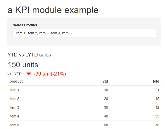
Let’s import a module to create a KPI widget. This module contains a function called “KPI_diff_pc_ModuleUI”.
This function takes a data frame as an input (for example a reactive data frame) with 2 numeric columns. It will then return a KPI object, to display the difference between 2 quantities, in value (amount) and in percentage.
In this example, the module is the R file “module_KPI_box.R”. It is stored on a GitHub repository.
We will download it using the function source() and the syntax : source("https://raw.githubusercontent.com/nguyennico/shiny_intro/main/module_KPI_box.R")
#----------------------# Upload libraries#----------------------# shinylibrary(shiny)library(shinyWidgets)# ETLlibrary(tidyverse)library(scales)# Tablelibrary(reactable)#----------------------# Upload Modules#----------------------# Source the R script from GitHub# source the modulesource("https://raw.githubusercontent.com/nguyennico/shiny_intro/main/module_KPI_box.R")#----------------------# Upload data or create datasets#----------------------product <-c("item 1", "item 2", "item 3", "item 4", "item 5")ytd <-c(10, 20, 30, 40, 50)lytd <-c(21, 15, 42, 33, 78)my_data <-data.frame(product, ytd, lytd)#----------------------# UI#----------------------ui <-fluidPage(headerPanel("a KPI module example"), # title of the appsidebarPanel(pickerInput("selected_product", "Select Product", choices =unique(as.character(my_data$product)),options =list(`actions-box`=TRUE),multiple = T,selected =unique(as.character(my_data$product))[1:20]#selected = c("item 1") # we also can preselect one or more value ) ), # close sidebarPanelmainPanel(KPI_diff_pc_ModuleUI("KPI_YTD_vs_LYTD"),reactableOutput("my_table") ) # close mainPanel) # close ui#----------------------# Server#----------------------server <-function(input, output) {#----------------------# Create Reactive#---------------------- my_reactive_data <-reactive({#------------------# Get data df1 <- my_data#------------------# Filters# select product df1 <- df1 |>filter(product %in% input$selected_product)#------------------# Tablereturn(df1) })#----------------------# Table 1#---------------------- output$my_table <-renderReactable({#------------------# Get data df1 <-my_reactive_data() df1 <-as.data.frame(df1)#------------------# Tablereactable(df1) })#----------------------# KPI 1# YTD vs LYTD#----------------------# call ModuleKPI_diff_pc_ModuleServer("KPI_YTD_vs_LYTD",data = my_reactive_data, previous ="lytd",new ="ytd",title ="YTD vs LYTD sales",subtitle ="vs LYTD :",uom ="units" )} # close servershinyApp(ui = ui, server = server)
In a nutshell : Using modules in R Shiny applications offers several benefits, particularly when it comes to organizing, maintaining, and scaling your applications.
Here are some key advantages:
Reusability:
Modules allow you to encapsulate functionality that can be reused across different parts of your application or even in different applications.
This reduces code duplication and makes it easier to maintain consistent behavior across your projects.
Encapsulation:
By using modules, you can encapsulate the internal workings of a component, exposing only the necessary inputs and outputs.
This leads to cleaner and more modular code, as each module can be developed and tested independently.
Scalability:
As your application grows, modules make it easier to scale by allowing you to add new features or modify existing ones without affecting other parts of the application.
This modular approach is particularly beneficial for large applications.
Maintenance, Debugging and Testing:
Modules can be developed and tested separately, which simplifies debugging.
You can isolate issues within a module without having to sift through the entire application code.
Collaboration:
When working in teams, modules allow different developers to work on different parts of the application simultaneously.
Each module can be assigned to different team members, facilitating parallel development.
56 Modern boostrap with bslib
What we have seen so far in terms of design is using Bootstrap 3. It’s the by default design of the shiny package. We can make it more modern, using the bslib package.
The bslib package in R is designed to enhance the styling and theming capabilities of Shiny applications by leveraging Bootstrap, a popular front-end framework.
Here are some advantages of using bslib:
Customizable Themes:
bslib allows to easily customize Bootstrap themes using variables such as colors, fonts, and spacing.
This enables us to create a unique look and feel for your shiny applications without needing extensive CSS knowledge.
Responsive Design:
Bootstrap is known for its responsive design capabilities, and bslib makes it easy to integrate these features into your shiny apps.
This ensures that our applications look good on a variety of devices, from desktops to tablets to smartphones.
Integration with Bootstrap 4 and 5:
bslib supports both Bootstrap 4 and 5, allowing you to leverage the latest features and improvements in the Bootstrap framework.
This includes new components, utilities, and improved grid systems.
Dynamic Theming:
You can create dynamic themes that change based on user input or other reactive conditions within your app.
This is useful for applications that need to adapt their appearance in real-time.
Easy to Use:
The package provides a user-friendly interface for theme customization, making it accessible even to those who are not familiar with web development.
Functions like bs_theme() and bs_add_variables() simplify the process of setting and modifying theme variables.
Enhanced Aesthetic Control:
With bslib, you have greater control over the aesthetics of your Shiny apps.
You can fine-tune aspects like typography, button styles, and layout, which can significantly improve the user experience.
To know more about bslib, let’s refer to the website of posit which presents it.