37  End to End (E2E)

38 Introduction

We’re going to see how to create an End to End (E2E) view, using the R package planr.

We will use a few functions from the package, especially to calculate projected inventories and a constrained demand.

Objective

Let’s consider 2 entities as follow:

• Entity 1 : is the receiver.

  • for ex.: a Market, a Distribution Center, a 3rd party wholesaler, etc…

• Entity 2 : is the supplier.

  • for ex.: a factory, a regional Distribution Center, etc…

Sales are performed by the Entity 1, which manages a local stock and gets a Supply from the Entity 2, which also holds one stock.

The Entity 1 :

• provides to the Entity 2 a Supply Plan, composed of Purchase Orders and Replenishment Forecasts.

• would like to know whether this Supply Plan will be delivered on time by the Entity 2 (the supplier).

At the same time, the Entity 2 would like to better understand the projected stocks of the Entity 1, to see whether there are any local risks in case of delays.

The purpose of the End-to-End (E2E) view is then to :

• provide a shared visibility on the projected inventories of both Entities.

• update the projected inventories of the Entity 1, considering the actual supply plan of the Entity 2.

Figure 67 : End to End (E2E) concept

38.1 Methodology

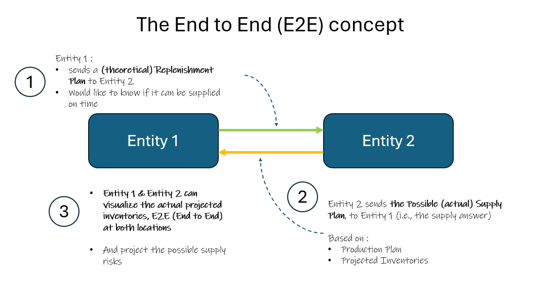
We will proceed in 3 steps :

• Step 1 : Get from the Entity 2 the actual Supplier’s answer.

  • Calculate the Entity 1’s projected inventories, and get the Constrained Demand, using the const_dmd() function from the R package planr.

  • Then translate this supply answer to the Entity 1, converting the ETD (Estimated Time of Departure) to the ETA (Estimated Time of Arrival).

• Step 2 : Calculate the projected in-transit.

  • always useful to get a total projection of the inventories, including the in-transit between the 2 entities.

• Step 3 : Update the Entity 1’s actual projected inventories.

  • based on the Constrained Supply ETA (= Constrained Demand from the Entity 2).

38.2 Inputs

From Entity 1 (the receiver), we need 5 variables :

• Sales Forecasts : in monthly or weekly bucket.

• Opening Stock On Hand.

• Supply Plan, usually composed of 3 variables :

  • Current in-transit.

    • with an ETA (Estimated Time of Arrival).

  • Pending Purchase Orders (POs).

    • with a theoretical arrival date, and shipment date (from the Entity 2, the supplier).

  • Future Replenishment Plan (forecasts, not necessarily materialized through a PO).

    • with a theoretical arrival date, and shipment date (from the Entity 2, the supplier).

Figure 68 : 3 usual variables of Supply to Entity 1

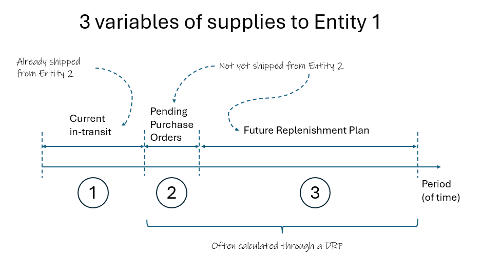
From Entity 2 (the supplier), we just need 2 variables :

• Opening Stock On Hand.

• Production Plan.

38.3 Master Data

We always need a few Master Data, they should especially cover :

• the Transit Lead Time,defined by SKU x Supplying Entity : let’s say 60 days here.

• eventually some SKUs Dimensions.

• a start date

start_date <- "2024-12-29"

start_date <- as.Date(start_date, format = "%Y-%m-%d")

start_date

[1] "2024-12-29"

38.4 Outputs

As a result of our calculation, we will get 3 standard outputs :

• For the Supplier (Entity 2) :

  • projected inventories and calculation of the constrained demand.

  • a cockpit (for a portfolio of products) : to visualize easily the OOS & Alerts, as well as the overstocks situations, at Supplier level.

• For the Receiver (Entity 1) :

  • actual projected inventories based on the constrained supply of the supplier.

• For both entities, an End to End (E2E) view :

  • displayed as a table with the projected inventories of both Entities next to each other.

  • a cockpit (for a portfolio of products) : to visualize easily the OOS & Alerts, as well as the overstocks situations, focusing on the Receiver (Entity 1) level.

As usual, we start by uploading the libraries we’re going to use :

# ETL
library(tidyverse)
library(sparkline)
library(htmltools)

# Charts
library(highcharter)

# Tables
library(reactable)
library(reactablefmtr)

# Supply Chain
library(planr)

39 Entity 1 (receiver)

Let’s a create a simple demo data frame, with only one product, called “Product A” .

It will contain 5 variables :

• Sales forecasts : initially in monthly bucket, that we will then split into weekly buckets.

• Opening Stock On Hand.

• a Supply Plan, composed of 3 elements :

  • Current in-transit.

  • Pending Purchase Orders (POs).

  • Future Replenishment Plan.

39.1 Dataset parts

Sales Forecasts

Let’s create some simple monthly sales forecasts, and then split them into weekly bucket :

# create variables and dataframe

Demand <- c(1000, 1000, 2000, 1000, 1000, 2000,
            1000, 1000, 2000, 1000, 1000, 2000)

Period <- c("2025-01-01", "2025-02-01", "2025-03-01", "2025-04-01", 
            "2025-05-01", "2025-06-01", "2025-07-01", "2025-08-01",
            "2025-09-01", "2025-10-01", "2025-11-01", "2025-12-01")

df1 <- data.frame(Period,
                  Demand)

# formatting
df1$Period <- as.Date(df1$Period, format = "%Y-%m-%d")

# add a DFU
df1$DFU <- "Product A"

glimpse(df1)

Rows: 12
Columns: 3
$ Period <date> 2025-01-01, 2025-02-01, 2025-03-01, 2025-04-01, 2025-05-01, 20…
$ Demand <dbl> 1000, 1000, 2000, 1000, 1000, 2000, 1000, 1000, 2000, 1000, 100…
$ DFU    <chr> "Product A", "Product A", "Product A", "Product A", "Product A"…

Now, let’s split those monthly Sales Forecasts into weekly bucket. We apply the function month_to_week() from the package planr.

By default, we consider the demand split evenly between different weeks.

Note : if we want a different pattern, we can use the function month_to_weekx().

# apply month_to_week()
df1 <- planr::month_to_week(dataset = df1, DFU, Period, Demand)

# formatting
df1$Period <- as.Date(df1$Period, format = "%Y-%m-%d")

# keep results
demand_data <- df1

glimpse(df1)

Rows: 53
Columns: 3
$ DFU    <chr> "Product A", "Product A", "Product A", "Product A", "Product A"…
$ Period <date> 2024-12-29, 2025-01-05, 2025-01-12, 2025-01-19, 2025-01-26, 20…
$ Demand <dbl> 142.8571, 250.0000, 250.0000, 250.0000, 142.8571, 250.0000, 250…

Opening Stock On Hand

Let’s put a random value, for example 1500 units.

We will affect this value to the first period of time, which is here the start_date (“2024-12-29”).

# create dataframe
df1 <- data.frame(
  DFU = c("Product A"),
  Period = c(start_date),
  Opening = 1500
  )

# keep results
opening_data <- df1

glimpse(df1)

Rows: 1
Columns: 3
$ DFU     <chr> "Product A"
$ Period  <date> 2024-12-29
$ Opening <dbl> 1500

Current in-transit

Let’s affect 2 random values, at ETA (Estimated Date of Arrival) :

• 600 units on the week of “2025-01-12”.

• 1200 units on the week of “2025-02-09”.

# create dataframe
df1 <- data.frame(
  DFU = c(rep("Product A", 2)),
  Period = c( "2025-01-12",  "2025-02-09"),
  In_transit = c(600, 1200)
  )

# formatting
df1$Period <- as.Date(df1$Period, format = "%Y-%m-%d")

# keep results
in_transit_data <- df1

glimpse(df1)

Rows: 2
Columns: 3
$ DFU        <chr> "Product A", "Product A"
$ Period     <date> 2025-01-12, 2025-02-09
$ In_transit <dbl> 600, 1200

Pending Purchase Orders (POs)

We affect 1 random value, at ETA (Estimated Date of Arrival) :

• 2000 units on the week of “2025-03-16”.

# create dataframe
df1 <- data.frame(
  DFU = c("Product A"),
  Period = c( "2025-03-16"),
  Pending_PO = c(2000)
  )

# formatting
df1$Period <- as.Date(df1$Period, format = "%Y-%m-%d")

# keep results
pending_po_data <- df1

glimpse(df1)

Rows: 1
Columns: 3
$ DFU        <chr> "Product A"
$ Period     <date> 2025-03-16
$ Pending_PO <dbl> 2000

Future Replenishment Plan

Now, let’s say that we have some monthly Replenishment Forecasts for the following 6 months, scheduled at some dates around the middle of each month.

# create dataframe
df1 <- data.frame(
  DFU = c(rep("Product A", 6)),
  Period = c( "2025-04-13",  "2025-05-11", "2025-06-15",
              "2025-07-13", "2025-08-17", "2025-09-14"),
  Replenishment_Plan = c(3000, 1000, 2000, 1000, 1000, 2000)
  )


# formatting
df1$Period <- as.Date(df1$Period, format = "%Y-%m-%d")

# keep results
replenishment_plan_data <- df1

glimpse(df1)

Rows: 6
Columns: 3
$ DFU                <chr> "Product A", "Product A", "Product A", "Product A",…
$ Period             <date> 2025-04-13, 2025-05-11, 2025-06-15, 2025-07-13, 20…
$ Replenishment_Plan <dbl> 3000, 1000, 2000, 1000, 1000, 2000

39.2 Create template

We are ready to combine those 3 parts (Demand | Opening | Supply) to get a template for the projected inventories of the Entity 1 :

# merge
df1 <- left_join(demand_data, opening_data)
df1 <- left_join(df1, in_transit_data)
df1 <- left_join(df1, pending_po_data)
df1 <- left_join(df1, replenishment_plan_data)

# replace missing values by zero
df1$Opening <- df1$Opening |> replace_na(0)
df1$In_transit <- df1$In_transit |> replace_na(0)
df1$Pending_PO <- df1$Pending_PO |> replace_na(0)
df1$Replenishment_Plan <- df1$Replenishment_Plan |> replace_na(0)

# calculate the total supply
df1$Supply <- df1$In_transit + df1$Pending_PO + df1$Replenishment_Plan

# keep results
Entity1_template_data <- df1

glimpse(df1)

Rows: 53
Columns: 8
$ DFU                <chr> "Product A", "Product A", "Product A", "Product A",…
$ Period             <date> 2024-12-29, 2025-01-05, 2025-01-12, 2025-01-19, 20…
$ Demand             <dbl> 142.8571, 250.0000, 250.0000, 250.0000, 142.8571, 2…
$ Opening            <dbl> 1500, 0, 0, 0, 0, 0, 0, 0, 0, 0, 0, 0, 0, 0, 0, 0, …
$ In_transit         <dbl> 0, 0, 600, 0, 0, 0, 1200, 0, 0, 0, 0, 0, 0, 0, 0, 0…
$ Pending_PO         <dbl> 0, 0, 0, 0, 0, 0, 0, 0, 0, 0, 0, 2000, 0, 0, 0, 0, …
$ Replenishment_Plan <dbl> 0, 0, 0, 0, 0, 0, 0, 0, 0, 0, 0, 0, 0, 0, 0, 3000, …
$ Supply             <dbl> 0, 0, 600, 0, 0, 0, 1200, 0, 0, 0, 0, 2000, 0, 0, 0…

39.3 Calculate Projected Inventories

Now, we’re going to calculate the theoretical projected inventories at the Entity 1 level.

Theoretical because we assume that all the planned quantities will be delivered on time. This is what we will need to verify this later on, using the End to End (E2E) view.

Let’s apply the function light_proj_inv() from the package planr :

# set a working df
df1 <- Entity1_template_data

# keep only needed variables
df1 <- df1 |> select(DFU, Period, Demand, Opening, Supply)

# calculate the projected inventories
df1 <- planr::light_proj_inv(dataset = df1, 
                             DFU = DFU, 
                             Period = Period,
                             Demand =  Demand, 
                             Opening = Opening, 
                             Supply = Supply)

# keep results
entity1_calculated_projection_data <- df1

glimpse(df1)

Rows: 53
Columns: 7
$ DFU                            <chr> "Product A", "Product A", "Product A", …
$ Period                         <date> 2024-12-29, 2025-01-05, 2025-01-12, 20…
$ Demand                         <dbl> 142.8571, 250.0000, 250.0000, 250.0000,…
$ Opening                        <dbl> 1500, 0, 0, 0, 0, 0, 0, 0, 0, 0, 0, 0, …
$ Calculated.Coverage.in.Periods <dbl> 5.9, 4.9, 6.1, 5.1, 4.1, 3.1, 4.5, 3.5,…
$ Projected.Inventories.Qty      <dbl> 1357.1, 1107.1, 1457.1, 1207.1, 1064.3,…
$ Supply                         <dbl> 0, 0, 600, 0, 0, 0, 1200, 0, 0, 0, 0, 2…

We can visualize the results using the libraries reactable and reactablefmtr :

#-------------------
# Get data
#-------------------

# set a working df
df1 <- entity1_calculated_projection_data


#-------------------
# Transform
#-------------------

# keep only the needed variables
df1 <- df1 |> select(Period,
                     Demand,
                     Calculated.Coverage.in.Periods,
                     Projected.Inventories.Qty,
                     Supply)


# create a f_colorpal field
df1 <- df1 |> mutate(f_colorpal = case_when(
  Calculated.Coverage.in.Periods > 6 ~ "#FFA500",
  Calculated.Coverage.in.Periods > 2 ~ "#32CD32",
  Calculated.Coverage.in.Periods > 0 ~ "#FFFF99",
  TRUE ~ "#FF0000" ))



#-------------------
# Table
#-------------------


# create reactable
reactable(df1, resizable = TRUE, showPageSizeOptions = TRUE,

              striped = TRUE, highlight = TRUE, compact = TRUE,
              defaultPageSize = 20,

              columns = list(

                Demand = colDef(
                  name = "Demand (units)",

                  cell = data_bars(df1,
                                   fill_color = "#3fc1c9",
                                   text_position = "outside-end"
                  )

                ),

              Calculated.Coverage.in.Periods = colDef(
                name = "Coverage (Periods)",
                maxWidth = 90,
                cell= color_tiles(df1, color_ref = "f_colorpal")
              ),

              f_colorpal = colDef(show = FALSE), # hidden, just used for the coverages

                `Projected.Inventories.Qty`= colDef(
                  name = "Projected Inventories (units)",
                  format = colFormat(separators = TRUE, digits=0),

                  style = function(value) {
                    if (value > 0) {
                      color <- "#008000"
                    } else if (value < 0) {
                      color <- "#e00000"
                    } else {
                      color <- "#777"
                    }
                    list(color = color
                         #fontWeight = "bold"
                    )
                  }
                ),

              Supply = colDef(
                name = "Supply (units)",
                cell = data_bars(df1,
                                 fill_color = "#3CB371",
                                 text_position = "outside-end"
                                 )
                )

              ), # close columns lits

              columnGroups = list(
                
                colGroup(name = "Projected Inventories", 
                         columns = c("Calculated.Coverage.in.Periods",
                                     "Projected.Inventories.Qty")
                         )
                )

    ) # close reactable

40 Entity 2 (supplier)

40.1 Dataset parts

Following the same approach, let’s a create a simple demo data frame, with only one product, called “Product A” .

It will contain 3 variables :

• Opening Stock On Hand.

• Production Plan.

• Demand forecasts : the expected supply from the Entity 1, excluding the current in transit, that we calculated previously.

Opening Stock On Hand

Let’s put a random value, for example 3000 units.

We will affect this value to the first period of time, which is here the start_date (“2024-12-29”).

# create dataframe
df1 <- data.frame(
  DFU = c("Product A"),
  Period = c(start_date),
  Opening = 3000
  )

# keep results
opening_data <- df1

glimpse(df1)

Rows: 1
Columns: 3
$ DFU     <chr> "Product A"
$ Period  <date> 2024-12-29
$ Opening <dbl> 3000

Production Plan

Let’s affect 3 random values, at different Production dates :

• 2000 units on the week of “2025-03-02”.

• 3000 units on the week of “2025-04-20”.

• 3000 units on the week of “2025-05-04”.

# create dataframe
df1 <- data.frame(
  DFU = c(rep("Product A", 3)),
  Period = c("2025-03-02", "2025-04-20", "2025-05-04"),
  Supply = c(2000, 3000, 3000)
  )

# formatting
df1$Period <- as.Date(df1$Period, format = "%Y-%m-%d")

# keep results
production_plan_data <- df1

glimpse(df1)

Rows: 3
Columns: 3
$ DFU    <chr> "Product A", "Product A", "Product A"
$ Period <date> 2025-03-02, 2025-04-20, 2025-05-04
$ Supply <dbl> 2000, 3000, 3000

Demand

The Demand to the Entity 2 is the expected supply from the Entity 1, excluding the current in transit :

• Pending Purchase Orders.

• Future Replenishment Plan.

So, first, let’s get those variables, at ETA date :

# set a working df
df1 <- Entity1_template_data

# keep only needed variables
df1 <- df1 |> select(DFU, Period, Pending_PO, Replenishment_Plan)

# calculate total demand
df1$Demand <- df1$Pending_PO + df1$Replenishment_Plan

# display
head(df1)

        DFU     Period Pending_PO Replenishment_Plan Demand
1 Product A 2024-12-29          0                  0      0
2 Product A 2025-01-05          0                  0      0
3 Product A 2025-01-12          0                  0      0
4 Product A 2025-01-19          0                  0      0
5 Product A 2025-01-26          0                  0      0
6 Product A 2025-02-02          0                  0      0

Now, we convert this ETA Demand into ETD date, using the transit leadtime.

We just need to offset the Demand by the transit leadtime (60days) .

Note :

• here we just write the transit leadtime inside the code, because we only have one product.

• if we have SKUs with different transit leadtimes, we need to have in our master data a dataset with the transit leadtimes by SKU and merge this dataset with the above table.

To keep it simple in this example, we just offset the transit leadtime straight in the original table

# offset of the transit leadtime
df1$Period <- df1$Period - 60 # because the transit lead time is 60 days

# make sure the new Period fits to the beginning of a week period
df1$Period <- floor_date(df1$Period, unit = "week")

# it's possible that the new ETD ends up on the similar weekly period
# so let's aggregate to avoid any issue
df1 <- df1 |> group_by(DFU, Period) |>
  summarise(Demand = sum(Demand)
            )

# keep only the relevant period of time
df1 <- df1 |> filter(Period >= start_date)

# keep results
demand_etd_data <- df1

# display
head(df1)

# A tibble: 6 × 3
# Groups:   DFU [1]
  DFU       Period     Demand
  <chr>     <date>      <dbl>
1 Product A 2024-12-29      0
2 Product A 2025-01-05      0
3 Product A 2025-01-12   2000
4 Product A 2025-01-19      0
5 Product A 2025-01-26      0
6 Product A 2025-02-02      0

40.2 Create template

Now let’s combine those 3 parts (Demand | Opening | Supply) to get a template to calculate the projected inventories and the Constrained Demand of the Entity 2 :

# merge
df1 <- left_join(demand_etd_data, opening_data)
df1 <- left_join(df1, production_plan_data)

# replace missing values by zero
df1$Opening <- df1$Opening |> replace_na(0)
df1$Supply <- df1$Supply |> replace_na(0)

# keep results
Entity2_template_data <- df1

# display
head(df1)

# A tibble: 6 × 5
# Groups:   DFU [1]
  DFU       Period     Demand Opening Supply
  <chr>     <date>      <dbl>   <dbl>  <dbl>
1 Product A 2024-12-29      0    3000      0
2 Product A 2025-01-05      0       0      0
3 Product A 2025-01-12   2000       0      0
4 Product A 2025-01-19      0       0      0
5 Product A 2025-01-26      0       0      0
6 Product A 2025-02-02      0       0      0

40.3 Calculate Constrained Demand

Let’s apply the function const_dmd() from the package planr.

# set a working df
df1 <- Entity2_template_data


# calculate the Proj Inv & Const Dmd
df1 <- planr::const_dmd(dataset = df1,
                        DFU = DFU,
                        Period = Period,
                        Demand =  Demand,
                        Opening = Opening,
                        Supply = Supply)


# keep results
entity2_calculated_projection_data <- df1

glimpse(df1)

Rows: 44
Columns: 9
$ DFU                            <chr> "Product A", "Product A", "Product A", …
$ Period                         <date> 2024-12-29, 2025-01-05, 2025-01-12, 20…
$ Demand                         <dbl> 0, 0, 2000, 0, 0, 0, 3000, 0, 0, 0, 100…
$ Opening                        <dbl> 3000, 0, 0, 0, 0, 0, 0, 0, 0, 0, 0, 0, …
$ Calculated.Coverage.in.Periods <dbl> 5.3, 4.3, 3.3, 2.3, 1.3, 0.3, 0.0, 0.0,…
$ Projected.Inventories.Qty      <dbl> 3000, 3000, 1000, 1000, 1000, 1000, -20…
$ Supply                         <dbl> 0, 0, 0, 0, 0, 0, 0, 0, 0, 2000, 0, 0, …
$ Constrained.Demand             <dbl> 0, 0, 2000, 0, 0, 0, 1000, 0, 0, 2000, …
$ Current.Stock.Available.Tag    <dbl> 0, 0, 1, 0, 0, 0, 0, 0, 0, 0, 0, 0, 0, …

As we just did for the Entity 1, we can visualize the results using the libraries reactable and reactablefmtr :

Let’s create a function status_badge() to display a badge :

# A Function to define a Badge Status in the reactable

status_badge <- function(color = "#aaa", width = "9px", height = width) {
  span(style = list(
    display = "inline-block",
    marginRight = "8px",
    width = width,
    height = height,
    backgroundColor = color,
    borderRadius = "50%"
  ))
}

Now let’s display the table :

# set a working df
df1 <- entity2_calculated_projection_data


#----------------
# Create the table
#----------------

# remove not needed column
df1 <- df1 |> select(-DFU)

    
# reorder variables
df1 <- df1 |> select(Period, Demand, Constrained.Demand, Current.Stock.Available.Tag,
                     Calculated.Coverage.in.Periods, Projected.Inventories.Qty, Supply
                     )
    
# create a f_colorpal field
df1 <- df1 |> mutate(f_colorpal = case_when(Calculated.Coverage.in.Periods > 6 ~ "#FFA500", 
                                            Calculated.Coverage.in.Periods > 2 ~ "#32CD32",
                                            Calculated.Coverage.in.Periods > 0 ~ "#FFFF99",
                                            TRUE ~ "#FF0000" ))
    
    
# adjust Current.Stock.Available.Tag
df1$Current.Stock.Available.Tag <- if_else(df1$Current.Stock.Available.Tag == 1, "Available", "")

    
#-------------------------
# Create Table
    
    
    
reactable(df1, resizable = TRUE, showPageSizeOptions = TRUE, 
              
              striped = TRUE, highlight = TRUE, compact = TRUE, 
              defaultPageSize = 20,
              
              columns = list(

                
                Demand = colDef(
                  name = "Demand (units)",
                  
                  cell = data_bars(df1,
                                   fill_color = "#3fc1c9",
                                   text_position = "outside-end")
                  
                ),
                
                Constrained.Demand = colDef(
                  
                  name = "Constrained Demand (units)",
                  
                  cell = data_bars(df1,
                                   fill_color = "gold",
                                   text_position = "outside-end")
                  
                ),
                

                
                Calculated.Coverage.in.Periods = colDef(
                  name = "Coverage (Periods)",
                  maxWidth = 90,
                  
                  cell= color_tiles(df1, color_ref = "f_colorpal")
                ),
                
                
                f_colorpal = colDef(show = FALSE), # hidden, just used for the coverages
                

                
                `Projected.Inventories.Qty`= colDef(
                  name = "Projected Inventories (units)",
                  format = colFormat(separators = TRUE, digits=0),
                  
                  style = function(value) {
                    if (value > 0) {
                      color <- "#008000"
                    } else if (value < 0) {
                      color <- "#e00000"
                    } else {
                      color <- "#777"
                    }
                    list(color = color
                         #fontWeight = "bold"
                    )
                  }
                ),
                
                
                Current.Stock.Available.Tag = colDef(
                  name = "Current Stock Available Tag",
                  
                  cell = function(value) {
                    color <- switch(
                      value,
                      No = "hsl(120,61%,50%)",
                      Available = "rgb(135,206,250)"
                    )
                    badge <- status_badge(color = color)
                    tagList(badge, value)
                  }),
                

                
                Supply = colDef(
                  name = "Supply (units)",
                  cell = data_bars(df1,
                                   fill_color = "#3CB371",
                                   text_position = "outside-end"
                  )
                )
                
                
 
                
              ), # close columns list
              
              columnGroups = list(
                
                colGroup(name = "Projected Inventories", 
                         columns = c("Calculated.Coverage.in.Periods", 
                                     "Projected.Inventories.Qty")
                         )
                )
              
    ) # close reactable

We can see that the Entity 2 will be late to supply the Demand coming from the Entity 1, from beginning of February until the end of April.

Creating the E2E view later on, we will figure out whether there is any significant impact at the Entity 1 level.

41 Projected In Transit

Now we’re going to project the In Transit inventories. There are 2 parts :

• current In Transit (already shipped).

• next In Transit (not yet shipped).

41.1 Current In Transit

Let’s use the current in transit at ETA date.

Opening GIT

We calculate the Opening In Transit, as the sum of all the quantities currently in transit.

# set a working df
df1 <- in_transit_data

# aggregate
df1 <- df1 |> group_by(DFU) |> 
  summarise(Current.GIT  = sum(In_transit)
            )

# Add Start.Date
df1$Period <- start_date

# keep results
opening_GIT_data <- df1

# display
df1

# A tibble: 1 × 3
  DFU       Current.GIT Period    
  <chr>           <dbl> <date>    
1 Product A        1800 2024-12-29

ETA Current GIT

Here, we identify the ETA (Estimated Time of Arrival) of those current In Transit inventories. We actually already have those info, and just rename the variable as ETA.Current.GIT.

We also add a tag, Tag.In.Transit, to better differentiate them, and highlight them in a table later on.

# set a working df
df1 <- in_transit_data

# add Current_GIT_DB
df1 <- left_join(df1, opening_GIT_data)

# replace missing values by zero
df1$Current.GIT <- df1$Current.GIT |> replace_na(0)

# rename
df1 <- df1 |> rename(ETA.Current.GIT = In_transit)

# add Tag.In.Transit
df1$Tag.In.Transit <- if_else(df1$ETA.Current.GIT > 0, "GIT", "")


# keep results
Current_GIT_data <- df1

# display
df1

        DFU     Period ETA.Current.GIT Current.GIT Tag.In.Transit
1 Product A 2025-01-12             600           0            GIT
2 Product A 2025-02-09            1200           0            GIT

41.2 Get Next In Transit

We will use the Entity 2’s Projected Inventories, with the calculated constrained demand.

Get ETD (Estimated Departure Date)

This is based on the Constrained Demand.

# set a working df
df1 <- entity2_calculated_projection_data

# keep only the needed variables
df1 <- df1 |> select(DFU, 
                     Period, 
                     Constrained.Demand, 
                     Current.Stock.Available.Tag)

# rename
df1 <- df1 |> rename(Supplier.Date = Period,
                     ETD.Future.In.Transit.Qty = Constrained.Demand,
                     Supplier.Current.Stock.Available.Tag = Current.Stock.Available.Tag
                     )


# keep Results
ETD_data <- df1

# display
head(df1)

        DFU Supplier.Date ETD.Future.In.Transit.Qty
1 Product A    2024-12-29                         0
2 Product A    2025-01-05                         0
3 Product A    2025-01-12                      2000
4 Product A    2025-01-19                         0
5 Product A    2025-01-26                         0
6 Product A    2025-02-02                         0
  Supplier.Current.Stock.Available.Tag
1                                    0
2                                    0
3                                    1
4                                    0
5                                    0
6                                    0

Get the related ETA

We need to consider the Transit Lead Time of each DFU.

In this example, we only have one transit Transit Lead Time : 60 days.

# set a working df
df1 <- ETD_data

# Add the Transit Times
df1$Transit.Time <- 60 # in days

# calculate the Receiver.Date
df1$Receiver.Date <- df1$Supplier.Date + df1$Transit.Time

# get start of the week day using lubridate
df1$Receiver.Date <- floor_date(df1$Receiver.Date, unit = "week")

# keep only needed variables
df1 <- df1 |> select(DFU, 
                     Receiver.Date, 
                     ETD.Future.In.Transit.Qty, 
                     Supplier.Current.Stock.Available.Tag)

# rename
df1 <- df1 |> rename(Period = Receiver.Date,
                     ETA.Future.In.Transit.Qty = ETD.Future.In.Transit.Qty,
                     Receiver.Current.Stock.Available.Tag = Supplier.Current.Stock.Available.Tag)

# aggregate
df1 <- df1 |> group_by(DFU, Period, Receiver.Current.Stock.Available.Tag) |> 
  summarise(ETA.Future.In.Transit.Qty = sum(ETA.Future.In.Transit.Qty))

# keep Results
ETA_data <- df1

glimpse(df1)

Rows: 44
Columns: 4
Groups: DFU, Period [44]
$ DFU                                  <chr> "Product A", "Product A", "Produc…
$ Period                               <date> 2025-02-23, 2025-03-02, 2025-03-…
$ Receiver.Current.Stock.Available.Tag <dbl> 0, 0, 1, 0, 0, 0, 0, 0, 0, 0, 0, …
$ ETA.Future.In.Transit.Qty            <dbl> 0, 0, 2000, 0, 0, 0, 1000, 0, 0, …

Combine ETD ETA

We get the final data frame with both ETD & ETA :

# rename
ETD_data <- ETD_data |> rename(Period = Supplier.Date)

# merge
df1 <- merge(ETD_data, ETA_data, all = TRUE)

# replace missing values by zero
df1$ETD.Future.In.Transit.Qty <- df1$ETD.Future.In.Transit.Qty |> replace_na(0)
df1$ETA.Future.In.Transit.Qty <- df1$ETA.Future.In.Transit.Qty |> replace_na(0)

# keep Results
ETD_ETA_data <- df1

glimpse(df1)

Rows: 52
Columns: 6
$ DFU                                  <chr> "Product A", "Product A", "Produc…
$ Period                               <date> 2024-12-29, 2025-01-05, 2025-01-…
$ ETD.Future.In.Transit.Qty            <dbl> 0, 0, 2000, 0, 0, 0, 1000, 0, 0, …
$ Supplier.Current.Stock.Available.Tag <dbl> 0, 0, 1, 0, 0, 0, 0, 0, 0, 0, 0, …
$ Receiver.Current.Stock.Available.Tag <dbl> NA, NA, NA, NA, NA, NA, NA, NA, 0…
$ ETA.Future.In.Transit.Qty            <dbl> 0, 0, 0, 0, 0, 0, 0, 0, 0, 0, 200…

41.3 Create In Transit template

We are going to combine 2 parts :

• Current In Transit, which contains the 2 variables :

  • Current GIT : i.e. the Opening In Transit.

  • ETA Current GIT.

• Future (or next) In Transit, which contains the 2 variables :

  • ETD.Next.GIT.

  • ETA.Next.GIT.

# merge
df1 <- merge(Current_GIT_data, ETD_ETA_data, all = TRUE)

# keep results
Interim_data <- df1

glimpse(df1)

Rows: 52
Columns: 9
$ DFU                                  <chr> "Product A", "Product A", "Produc…
$ Period                               <date> 2024-12-29, 2025-01-05, 2025-01-…
$ ETA.Current.GIT                      <dbl> NA, NA, 600, NA, NA, NA, 1200, NA…
$ Current.GIT                          <dbl> NA, NA, 0, NA, NA, NA, 0, NA, NA,…
$ Tag.In.Transit                       <chr> NA, NA, "GIT", NA, NA, NA, "GIT",…
$ ETD.Future.In.Transit.Qty            <dbl> 0, 0, 2000, 0, 0, 0, 1000, 0, 0, …
$ Supplier.Current.Stock.Available.Tag <dbl> 0, 0, 1, 0, 0, 0, 0, 0, 0, 0, 0, …
$ Receiver.Current.Stock.Available.Tag <dbl> NA, NA, NA, NA, NA, NA, NA, NA, 0…
$ ETA.Future.In.Transit.Qty            <dbl> 0, 0, 0, 0, 0, 0, 0, 0, 0, 0, 200…

We will add the Transit Time and express it in weeks to create a template for the In Transit.

We’ll call it In_Transit_data .

# Add the Transit Times
df1$Transit.Time <- 60 # in days


# keep only needed variables
df1 <- df1 |> select(DFU,
                     Period,
                     Current.GIT, 
                     ETA.Current.GIT,
                     ETD.Future.In.Transit.Qty, 
                     ETA.Future.In.Transit.Qty,
                     Transit.Time
                     )


# rename
df1 <- df1 |> rename(ETD.Next.GIT = ETD.Future.In.Transit.Qty,
                     ETA.Next.GIT = ETA.Future.In.Transit.Qty)


# convert the Transit.Time in weeks
df1$Transit.Time <- df1$Transit.Time / 7

# round
df1$Transit.Time <- round(df1$Transit.Time)

# keep results
In_Transit_data <- df1

glimpse(df1)

Rows: 52
Columns: 7
$ DFU             <chr> "Product A", "Product A", "Product A", "Product A", "P…
$ Period          <date> 2024-12-29, 2025-01-05, 2025-01-12, 2025-01-19, 2025-…
$ Current.GIT     <dbl> NA, NA, 0, NA, NA, NA, 0, NA, NA, NA, NA, NA, NA, NA, …
$ ETA.Current.GIT <dbl> NA, NA, 600, NA, NA, NA, 1200, NA, NA, NA, NA, NA, NA,…
$ ETD.Next.GIT    <dbl> 0, 0, 2000, 0, 0, 0, 1000, 0, 0, 2000, 0, 0, 0, 0, 0, …
$ ETA.Next.GIT    <dbl> 0, 0, 0, 0, 0, 0, 0, 0, 0, 0, 2000, 0, 0, 0, 1000, 0, …
$ Transit.Time    <dbl> 9, 9, 9, 9, 9, 9, 9, 9, 9, 9, 9, 9, 9, 9, 9, 9, 9, 9, …

41.4 Calculation In Transit

First, let’s get the ETD of the current In Transit.

Get & Add ETD.Current.GIT

# set a working df
df1 <- In_Transit_data

# calculate the ETD.Period
df1$ETD.Period <- df1$Period - (df1$Transit.Time * 7)

# keep only needed variables
df1 <- df1 |> select(DFU,
                     ETD.Period, 
                     ETA.Current.GIT)

# rename
df1 <- df1 |> rename(Period = ETD.Period,
                     ETD.Current.GIT = ETA.Current.GIT)

# get the beginning of the week for the Period
# to ensure we are following an english standard
df1$Period <- floor_date(df1$Period, unit = "week")

# aggregate
df1 <- df1 |> group_by(DFU, Period) |> 
  summarise(ETD.Current.GIT = sum(ETD.Current.GIT))



# add back to initial dataset
df1 <- merge(In_Transit_data, df1, all = TRUE)


# replace missing values by zero
df1$ETA.Current.GIT <- df1$ETA.Current.GIT |> replace_na(0)
df1$ETD.Current.GIT <- df1$ETD.Current.GIT |> replace_na(0)


# keep results
Interim_data <- df1

glimpse(df1)

Rows: 61
Columns: 8
$ DFU             <chr> "Product A", "Product A", "Product A", "Product A", "P…
$ Period          <date> 2024-10-27, 2024-11-03, 2024-11-10, 2024-11-17, 2024-…
$ Current.GIT     <dbl> NA, NA, NA, NA, NA, NA, NA, NA, NA, NA, NA, 0, NA, NA,…
$ ETA.Current.GIT <dbl> 0, 0, 0, 0, 0, 0, 0, 0, 0, 0, 0, 600, 0, 0, 0, 1200, 0…
$ ETD.Next.GIT    <dbl> NA, NA, NA, NA, NA, NA, NA, NA, NA, 0, 0, 2000, 0, 0, …
$ ETA.Next.GIT    <dbl> NA, NA, NA, NA, NA, NA, NA, NA, NA, 0, 0, 0, 0, 0, 0, …
$ Transit.Time    <dbl> NA, NA, NA, NA, NA, NA, NA, NA, NA, 9, 9, 9, 9, 9, 9, …
$ ETD.Current.GIT <dbl> 0, 0, 600, 0, 0, 0, 1200, 0, 0, 0, 0, 0, 0, 0, 0, 0, 0…

Calculate Projection Current GIT

Now let’s project the current In Transit.

# set a working df
df1 <- Interim_data


# accumulate data
df1 <- df1 |> group_by(DFU, Period) |>
    summarise(
      ETA.Current.GIT = sum(ETA.Current.GIT),
      ETD.Current.GIT = sum(ETD.Current.GIT)
      ) |>
  
    mutate(
      acc_ETA.Current.GIT = cumsum(ETA.Current.GIT),
      acc_ETD.Current.GIT = cumsum(ETD.Current.GIT)
    )

# calculate projected Current In Transit
df1$Proj.Current.GIT <- df1$acc_ETD.Current.GIT - df1$acc_ETA.Current.GIT


# keep only needed columns
df1 <- df1 |> select(DFU, Period, Proj.Current.GIT)

# keep Results
Proj_Current_In_Transit_data <- df1

glimpse(df1)

Rows: 61
Columns: 3
Groups: DFU [1]
$ DFU              <chr> "Product A", "Product A", "Product A", "Product A", "…
$ Period           <date> 2024-10-27, 2024-11-03, 2024-11-10, 2024-11-17, 2024…
$ Proj.Current.GIT <dbl> 0, 0, 600, 600, 600, 600, 1800, 1800, 1800, 1800, 180…

Calculate Projection Future GIT

Following the same methodology, we can project the future In Transit.

# set a working df
df1 <- In_Transit_data


# accumulate data
df1 <- df1 |> group_by(DFU, Period) |> 
  summarise(
      ETD.Next.GIT = sum(ETD.Next.GIT),
      ETA.Next.GIT = sum(ETA.Next.GIT)
      ) |>
  
    mutate(
      acc_ETD.Next.GIT = cumsum(ETD.Next.GIT),
      acc_ETA.Next.GIT = cumsum(ETA.Next.GIT)
    )


# calculate projected Future In Transit
df1$Proj.Future.GIT <- if_else(df1$acc_ETD.Next.GIT > df1$acc_ETA.Next.GIT,
                                          df1$acc_ETD.Next.GIT - df1$acc_ETA.Next.GIT,
                                          0)


# keep only needed columns
df1 <- df1 |> select(DFU, Period, Proj.Future.GIT)


# keep Results
Proj_Future_In_Transit_data <- df1

glimpse(df1)

Rows: 52
Columns: 3
Groups: DFU [1]
$ DFU             <chr> "Product A", "Product A", "Product A", "Product A", "P…
$ Period          <date> 2024-12-29, 2025-01-05, 2025-01-12, 2025-01-19, 2025-…
$ Proj.Future.GIT <dbl> 0, 0, 2000, 2000, 2000, 2000, 3000, 3000, 3000, 5000, …

Combine

Now we can combine the 3 parts :

• Opening In Transit.

• projected current In Transit.

• projected next In transit.

# merge everything
df1 <- left_join(Interim_data, Proj_Current_In_Transit_data)
df1 <- left_join(df1, Proj_Future_In_Transit_data)

# replace missing values by zero
df1$ETA.Current.GIT <- df1$ETA.Current.GIT |> replace_na(0)
df1$ETA.Next.GIT <- df1$ETA.Next.GIT |> replace_na(0)
df1$ETD.Next.GIT <- df1$ETD.Next.GIT |> replace_na(0)
df1$Current.GIT <- df1$Current.GIT |> replace_na(0)

df1$ETD.Current.GIT <- df1$ETD.Current.GIT |> replace_na(0)
df1$Proj.Current.GIT <- df1$Proj.Current.GIT |> replace_na(0)
df1$Proj.Future.GIT <- df1$Proj.Future.GIT |> replace_na(0)

# Calculate Total Projected In Transit
df1$Proj.GIT <- df1$Proj.Current.GIT + df1$Proj.Future.GIT


# keep only relevant Periods, i.e. > Start Date
df1 <- filter(df1, df1$Period >= start_date)

# formatting
df1 <- as.data.frame(df1)

# keep results
Projected_GIT_data <- df1

glimpse(df1)

Rows: 52
Columns: 11
$ DFU              <chr> "Product A", "Product A", "Product A", "Product A", "…
$ Period           <date> 2024-12-29, 2025-01-05, 2025-01-12, 2025-01-19, 2025…
$ Current.GIT      <dbl> 0, 0, 0, 0, 0, 0, 0, 0, 0, 0, 0, 0, 0, 0, 0, 0, 0, 0,…
$ ETA.Current.GIT  <dbl> 0, 0, 600, 0, 0, 0, 1200, 0, 0, 0, 0, 0, 0, 0, 0, 0, …
$ ETD.Next.GIT     <dbl> 0, 0, 2000, 0, 0, 0, 1000, 0, 0, 2000, 0, 0, 0, 0, 0,…
$ ETA.Next.GIT     <dbl> 0, 0, 0, 0, 0, 0, 0, 0, 0, 0, 2000, 0, 0, 0, 1000, 0,…
$ Transit.Time     <dbl> 9, 9, 9, 9, 9, 9, 9, 9, 9, 9, 9, 9, 9, 9, 9, 9, 9, 9,…
$ ETD.Current.GIT  <dbl> 0, 0, 0, 0, 0, 0, 0, 0, 0, 0, 0, 0, 0, 0, 0, 0, 0, 0,…
$ Proj.Current.GIT <dbl> 1800, 1800, 1200, 1200, 1200, 1200, 0, 0, 0, 0, 0, 0,…
$ Proj.Future.GIT  <dbl> 0, 0, 2000, 2000, 2000, 2000, 3000, 3000, 3000, 5000,…
$ Proj.GIT         <dbl> 1800, 1800, 3200, 3200, 3200, 3200, 3000, 3000, 3000,…

42 Entity 1 Actual Projected Inventories

42.1 Create new Entity 1 template

This time we will consider the actual (i.e. constrained) supply plan, based on the Entity 2’s supply answer.

We will create a template to calculate the actual projected inventories considering :

• the ETA of the constrained supply.

• the initial Sales Forecasts and Opening Inventories.

We will also add the info about Current.Stock.Available.Tag.

Get Const Supply

From an ETA (Estimated Time of Arrival) perspective.

# set a working df
df1 <- Projected_GIT_data

# get supply
df1$Supply <- df1$ETA.Current.GIT + df1$ETA.Next.GIT

# keep only needed variables
df1 <- df1 |> select(DFU,
                     Period,
                     Supply)

# keep results
const_supply_data <- df1

# display
head(df1)

        DFU     Period Supply
1 Product A 2024-12-29      0
2 Product A 2025-01-05      0
3 Product A 2025-01-12    600
4 Product A 2025-01-19      0
5 Product A 2025-01-26      0
6 Product A 2025-02-02      0

Get Sales Forecasts & Opening

They are the initial data, so we simply use the data frame Entity1_template_data .

# set a working df
df1 <- Entity1_template_data

# keep only needed variables
df1 <- df1 |> select(DFU, Period, Demand, Opening)

# display
head(df1)

        DFU     Period   Demand Opening
1 Product A 2024-12-29 142.8571    1500
2 Product A 2025-01-05 250.0000       0
3 Product A 2025-01-12 250.0000       0
4 Product A 2025-01-19 250.0000       0
5 Product A 2025-01-26 142.8571       0
6 Product A 2025-02-02 250.0000       0

Assemble

We assemble those 2 components.

# merge
df1 <- left_join(df1, const_supply_data)

# display
head(df1)

        DFU     Period   Demand Opening Supply
1 Product A 2024-12-29 142.8571    1500      0
2 Product A 2025-01-05 250.0000       0      0
3 Product A 2025-01-12 250.0000       0    600
4 Product A 2025-01-19 250.0000       0      0
5 Product A 2025-01-26 142.8571       0      0
6 Product A 2025-02-02 250.0000       0      0

42.2 Calculate Entity 1 Projected Inventories

To calculate, we use the function light_proj_inv() from the package planr .

# calculate
df1 <- planr::light_proj_inv(data = df1, 
                             DFU = DFU, 
                             Period = Period, 
                             Demand =  Demand, 
                             Opening = Opening, 
                             Supply = Supply)

# keep results
Calculated_Entity1_Const_Proj_Inv_data <- df1

glimpse(df1)

Rows: 53
Columns: 7
$ DFU                            <chr> "Product A", "Product A", "Product A", …
$ Period                         <date> 2024-12-29, 2025-01-05, 2025-01-12, 20…
$ Demand                         <dbl> 142.8571, 250.0000, 250.0000, 250.0000,…
$ Opening                        <dbl> 1500, 0, 0, 0, 0, 0, 0, 0, 0, 0, 0, 0, …
$ Calculated.Coverage.in.Periods <dbl> 5.9, 4.9, 6.1, 5.1, 4.1, 3.1, 4.5, 3.5,…
$ Projected.Inventories.Qty      <dbl> 1357.1, 1107.1, 1457.1, 1207.1, 1064.3,…
$ Supply                         <dbl> 0, 0, 600, 0, 0, 0, 1200, 0, 0, 0, 2000…

Add Current Stocks available Tag

Now we add back the info about Current.Stock.Available.Tag, using the data frame ETD_ETA_data .

# set a working df
df1 <- ETD_ETA_data


# replace missing values by zero
df1$Receiver.Current.Stock.Available.Tag <- df1$Receiver.Current.Stock.Available.Tag |> replace_na(0)


# keep only unique values
df1 <- unique(df1)


# merge
df1 <- left_join(Calculated_Entity1_Const_Proj_Inv_data, df1)


# replace missing values by zero
df1$Receiver.Current.Stock.Available.Tag <- df1$Receiver.Current.Stock.Available.Tag |> replace_na(0)


# keep results
Calculated_Entity1_Const_Proj_Inv_data <- df1

glimpse(df1)

Rows: 53
Columns: 11
$ DFU                                  <chr> "Product A", "Product A", "Produc…
$ Period                               <date> 2024-12-29, 2025-01-05, 2025-01-…
$ Demand                               <dbl> 142.8571, 250.0000, 250.0000, 250…
$ Opening                              <dbl> 1500, 0, 0, 0, 0, 0, 0, 0, 0, 0, …
$ Calculated.Coverage.in.Periods       <dbl> 5.9, 4.9, 6.1, 5.1, 4.1, 3.1, 4.5…
$ Projected.Inventories.Qty            <dbl> 1357.1, 1107.1, 1457.1, 1207.1, 1…
$ Supply                               <dbl> 0, 0, 600, 0, 0, 0, 1200, 0, 0, 0…
$ ETD.Future.In.Transit.Qty            <dbl> 0, 0, 2000, 0, 0, 0, 1000, 0, 0, …
$ Supplier.Current.Stock.Available.Tag <dbl> 0, 0, 1, 0, 0, 0, 0, 0, 0, 0, 0, …
$ Receiver.Current.Stock.Available.Tag <dbl> 0, 0, 0, 0, 0, 0, 0, 0, 0, 0, 1, …
$ ETA.Future.In.Transit.Qty            <dbl> 0, 0, 0, 0, 0, 0, 0, 0, 0, 0, 200…

43 Create E2E

Here comes the last part to create the E2E view. We simply need to combine 3 blocks, related to :

• the Receiver.

• the Supplier.

• the In Transit.

Prepare Receiver

We’re going to keep especially the variables :

• sales forecasts.

• calculated (actual) projected inventories and coverage.

• (actual) supply plan from the supplier.

# set a working df
df1 <- Calculated_Entity1_Const_Proj_Inv_data

# rename
df1 <- df1 |> rename(
      sales_forecasts_qty = Demand,
      Receiver_opening_qty = Opening,
      Receiver_Calculated.Coverage.in.Periods = Calculated.Coverage.in.Periods,
      Receiver_Projected.Inventories.Qty  = Projected.Inventories.Qty,
      Receiver_Supply_qty = Supply
    )

# keep results
Receiver_PI_data <- df1

glimpse(df1)

Rows: 53
Columns: 11
$ DFU                                     <chr> "Product A", "Product A", "Pro…
$ Period                                  <date> 2024-12-29, 2025-01-05, 2025-…
$ sales_forecasts_qty                     <dbl> 142.8571, 250.0000, 250.0000, …
$ Receiver_opening_qty                    <dbl> 1500, 0, 0, 0, 0, 0, 0, 0, 0, …
$ Receiver_Calculated.Coverage.in.Periods <dbl> 5.9, 4.9, 6.1, 5.1, 4.1, 3.1, …
$ Receiver_Projected.Inventories.Qty      <dbl> 1357.1, 1107.1, 1457.1, 1207.1…
$ Receiver_Supply_qty                     <dbl> 0, 0, 600, 0, 0, 0, 1200, 0, 0…
$ ETD.Future.In.Transit.Qty               <dbl> 0, 0, 2000, 0, 0, 0, 1000, 0, …
$ Supplier.Current.Stock.Available.Tag    <dbl> 0, 0, 1, 0, 0, 0, 0, 0, 0, 0, …
$ Receiver.Current.Stock.Available.Tag    <dbl> 0, 0, 0, 0, 0, 0, 0, 0, 0, 0, …
$ ETA.Future.In.Transit.Qty               <dbl> 0, 0, 0, 0, 0, 0, 0, 0, 0, 0, …

Prepare Supplier

In a similar way, we’re going to keep the following variables :

• 2 general ones : DFU and Period of time.

• related to the Demand :

  • initial demand from the receiving entity.

  • constrained demand.

  • tag Current.Stock.Available.Tag.

• calculated projected inventories and coverage.

• related to the Opening and Supply.

# set a working df
df1 <- entity2_calculated_projection_data


# keep only needed variables
df1 <- df1 |> select(DFU ,
                     Period,
                     Demand,
                     Constrained.Demand,
                     Current.Stock.Available.Tag,
                     Calculated.Coverage.in.Periods,
                     Projected.Inventories.Qty,
                     Opening,
                     Supply)


# rename
df1 <- df1 |> rename(
      Supplier_Total.Demand_qty = Demand,
      Supplier_Confirmed.Supply.Plan_qty = Constrained.Demand,
      Supplier_Current.Stock.Available.Tag = Current.Stock.Available.Tag,
      Supplier_Opening_qty = Opening,
      Supplier_Calculated.Coverage.in.Periods = Calculated.Coverage.in.Periods,
      Supplier_Projected.Inventories.Qty  = Projected.Inventories.Qty,
      Supplier_Supply_qty = Supply
    )

# keep results
Supplier_PI_data <- df1

glimpse(df1)

Rows: 44
Columns: 9
$ DFU                                     <chr> "Product A", "Product A", "Pro…
$ Period                                  <date> 2024-12-29, 2025-01-05, 2025-…
$ Supplier_Total.Demand_qty               <dbl> 0, 0, 2000, 0, 0, 0, 3000, 0, …
$ Supplier_Confirmed.Supply.Plan_qty      <dbl> 0, 0, 2000, 0, 0, 0, 1000, 0, …
$ Supplier_Current.Stock.Available.Tag    <dbl> 0, 0, 1, 0, 0, 0, 0, 0, 0, 0, …
$ Supplier_Calculated.Coverage.in.Periods <dbl> 5.3, 4.3, 3.3, 2.3, 1.3, 0.3, …
$ Supplier_Projected.Inventories.Qty      <dbl> 3000, 3000, 1000, 1000, 1000, …
$ Supplier_Opening_qty                    <dbl> 3000, 0, 0, 0, 0, 0, 0, 0, 0, …
$ Supplier_Supply_qty                     <dbl> 0, 0, 0, 0, 0, 0, 0, 0, 0, 200…

Prepare In Transit

Now we will create a data frame related to the In Transit inventories. It will contain the following variables :

• 2 general ones : DFU and Period of time.

• parts related to the current In Transit :

  • Current.GIT and ETA.Current.GIT.

• parts related to the next In Transit :

  • ETD.Next.GIT and ETA.Next.GIT.

• projected In Transit :

  • Proj.Current.GIT, Proj.Future.GIT and Proj.GIT.

The 2 first parts will provide an understanding of the supply plan : when and how much will be shipped, and when it will arrive.

The projected In Transit part will be useful to project the total stocks, especially summing the 3 values : at Supplier side, Receiver side, and in between, the in-transit.

# set a working df
df1 <- Projected_GIT_data

# keep only needed variables
df1 <- df1 |> select(DFU,
                     Period,
                     Current.GIT,
                     ETA.Current.GIT,
                     ETD.Next.GIT,
                     ETA.Next.GIT,
                     
                     Proj.Current.GIT,
                     Proj.Future.GIT,
                     Proj.GIT)


# keep results
GIT_data <- df1

glimpse(df1)

Rows: 52
Columns: 9
$ DFU              <chr> "Product A", "Product A", "Product A", "Product A", "…
$ Period           <date> 2024-12-29, 2025-01-05, 2025-01-12, 2025-01-19, 2025…
$ Current.GIT      <dbl> 0, 0, 0, 0, 0, 0, 0, 0, 0, 0, 0, 0, 0, 0, 0, 0, 0, 0,…
$ ETA.Current.GIT  <dbl> 0, 0, 600, 0, 0, 0, 1200, 0, 0, 0, 0, 0, 0, 0, 0, 0, …
$ ETD.Next.GIT     <dbl> 0, 0, 2000, 0, 0, 0, 1000, 0, 0, 2000, 0, 0, 0, 0, 0,…
$ ETA.Next.GIT     <dbl> 0, 0, 0, 0, 0, 0, 0, 0, 0, 0, 2000, 0, 0, 0, 1000, 0,…
$ Proj.Current.GIT <dbl> 1800, 1800, 1200, 1200, 1200, 1200, 0, 0, 0, 0, 0, 0,…
$ Proj.Future.GIT  <dbl> 0, 0, 2000, 2000, 2000, 2000, 3000, 3000, 3000, 5000,…
$ Proj.GIT         <dbl> 1800, 1800, 3200, 3200, 3200, 3200, 3000, 3000, 3000,…

Create E2E incl. Transit

We simply combine the 3 parts we created.

#-------------------------------------
# Merge Receiver and Supplier Projected Inventories
#-------------------------------------

# merge
df1 <- left_join(Supplier_PI_data, Receiver_PI_data)


#-------------------------------------
# Add In Transit
#-------------------------------------

# merge
df1 <- left_join(df1, GIT_data)


# keep results
Set_Up_E2E_data <- df1

glimpse(df1)

Rows: 44
Columns: 25
$ DFU                                     <chr> "Product A", "Product A", "Pro…
$ Period                                  <date> 2024-12-29, 2025-01-05, 2025-…
$ Supplier_Total.Demand_qty               <dbl> 0, 0, 2000, 0, 0, 0, 3000, 0, …
$ Supplier_Confirmed.Supply.Plan_qty      <dbl> 0, 0, 2000, 0, 0, 0, 1000, 0, …
$ Supplier_Current.Stock.Available.Tag    <dbl> 0, 0, 1, 0, 0, 0, 0, 0, 0, 0, …
$ Supplier_Calculated.Coverage.in.Periods <dbl> 5.3, 4.3, 3.3, 2.3, 1.3, 0.3, …
$ Supplier_Projected.Inventories.Qty      <dbl> 3000, 3000, 1000, 1000, 1000, …
$ Supplier_Opening_qty                    <dbl> 3000, 0, 0, 0, 0, 0, 0, 0, 0, …
$ Supplier_Supply_qty                     <dbl> 0, 0, 0, 0, 0, 0, 0, 0, 0, 200…
$ sales_forecasts_qty                     <dbl> 142.8571, 250.0000, 250.0000, …
$ Receiver_opening_qty                    <dbl> 1500, 0, 0, 0, 0, 0, 0, 0, 0, …
$ Receiver_Calculated.Coverage.in.Periods <dbl> 5.9, 4.9, 6.1, 5.1, 4.1, 3.1, …
$ Receiver_Projected.Inventories.Qty      <dbl> 1357.1, 1107.1, 1457.1, 1207.1…
$ Receiver_Supply_qty                     <dbl> 0, 0, 600, 0, 0, 0, 1200, 0, 0…
$ ETD.Future.In.Transit.Qty               <dbl> 0, 0, 2000, 0, 0, 0, 1000, 0, …
$ Supplier.Current.Stock.Available.Tag    <dbl> 0, 0, 1, 0, 0, 0, 0, 0, 0, 0, …
$ Receiver.Current.Stock.Available.Tag    <dbl> 0, 0, 0, 0, 0, 0, 0, 0, 0, 0, …
$ ETA.Future.In.Transit.Qty               <dbl> 0, 0, 0, 0, 0, 0, 0, 0, 0, 0, …
$ Current.GIT                             <dbl> 0, 0, 0, 0, 0, 0, 0, 0, 0, 0, …
$ ETA.Current.GIT                         <dbl> 0, 0, 600, 0, 0, 0, 1200, 0, 0…
$ ETD.Next.GIT                            <dbl> 0, 0, 2000, 0, 0, 0, 1000, 0, …
$ ETA.Next.GIT                            <dbl> 0, 0, 0, 0, 0, 0, 0, 0, 0, 0, …
$ Proj.Current.GIT                        <dbl> 1800, 1800, 1200, 1200, 1200, …
$ Proj.Future.GIT                         <dbl> 0, 0, 2000, 2000, 2000, 2000, …
$ Proj.GIT                                <dbl> 1800, 1800, 3200, 3200, 3200, …

44 E2E Visuals

Let’s visualize our E2E table using the libraries reactable and reactablefmtr.

First, let’s create the data frame we aim to display :

• we follow a classic 4 steps approach : Get data => Filter => Transform => display Table.

• to make the horizon shorter we will filter the horizon before “2025-06-30”.

We also organize here the flow of the table :

• on the right the supplying entity.

• on the left the receiving entity.

• in the middle the in-transit inventories.

And we do a little bit of formatting, especially for the projected coverages.

#------------------------------
# Get data
df1 <- Set_Up_E2E_data
    

#------------------------------
# Filter
    
# filter Period to display a shorter horizon
df1 <- df1 |> filter(Period <= "2025-06-30")
    
    
#------------------------------
# Transform
    
# keep only needed variables
df1 <- df1 |> select(Period,
                     
                     #-------------
                     # Receiver part
                     sales_forecasts_qty,
                     Receiver_Calculated.Coverage.in.Periods,
                     Receiver_Projected.Inventories.Qty,
                     
                     #-------------
                     # In Transit part
                     ETA.Current.GIT,
                     ETA.Next.GIT,
                     Receiver.Current.Stock.Available.Tag,
                     
                     #-------------
                     # Supplier part
                     Supplier_Total.Demand_qty,
                     Supplier_Confirmed.Supply.Plan_qty,
                     
                     Supplier_Calculated.Coverage.in.Periods,
                     Supplier_Projected.Inventories.Qty,
                     Supplier_Supply_qty
                     )
    
    
    
# format Coverage at one digit after comma 
df1$Receiver_Calculated.Coverage.in.Periods <- format(round(df1$Receiver_Calculated.Coverage.in.Periods, 1), nsmall = 1)
    
df1$Supplier_Calculated.Coverage.in.Periods <- format(round(df1$Supplier_Calculated.Coverage.in.Periods, 1), nsmall = 1)
    
    
# replace Current Stock Available Tag from numerical to characters
df1$Receiver.Current.Stock.Available.Tag <- if_else(df1$Receiver.Current.Stock.Available.Tag == 1, "ok", "")
    
    
#-----------------
# create a f_colorpal field
#-----------------
    
#-----------------
# for Receiver
    
# formatting
df1$Receiver_Calculated.Coverage.in.Periods <- as.numeric(df1$Receiver_Calculated.Coverage.in.Periods)
    
# create f_colorpal field
df1 <- df1 |> mutate(
  Receiver_f_colorpal = case_when(
    Receiver_Calculated.Coverage.in.Periods > 16 ~ "lightblue",
    Receiver_Calculated.Coverage.in.Periods > 4 ~ "white",
    Receiver_Calculated.Coverage.in.Periods > 0 ~ "yellow",
    Receiver_Calculated.Coverage.in.Periods <= 0 ~ "tomato",
    TRUE ~ "#FFFFFF"))
    
    
    
#-----------------
# for Supplier
    
# formatting
df1$Supplier_Calculated.Coverage.in.Periods <- as.numeric(df1$Supplier_Calculated.Coverage.in.Periods)
    
# create f_colorpal field
df1 <- df1 |> mutate(
  Supplier_f_colorpal = case_when(
    Supplier_Calculated.Coverage.in.Periods > 16 ~ "lightblue",
    Supplier_Calculated.Coverage.in.Periods > 4 ~ "white",
    Supplier_Calculated.Coverage.in.Periods > 0 ~ "yellow",
    TRUE ~ "#FF0000" ))
    
    

# formatting for a better display
df1$sales_forecasts_qty <- as.integer(df1$sales_forecasts_qty)

Now we’re ready to created the E2E reactable.

We can notice that despite the fact that the Entity 2 will be late to supply, with some backorders in February, there won’t be, until June, any risk of shortage at the Entity 1 level.

An E2E view is then very useful to :

• provide a shared visibility on the projected inventories of both Entities.

• update the projected inventories of a receiving entity, considering the actual supply plan of the supplier.

#-------------------------
# Create Table
    
reactable(df1, 
          resizable = TRUE, 
          showPageSizeOptions = TRUE,
          striped = TRUE, highlight = TRUE, compact = TRUE,
          defaultPageSize = 50,
          
          
          columns = list(
            
            Period = colDef(
              name = "Period",
              sticky = "left"),
            
            
            #------------------------
            # Receiver
            
            
            
            sales_forecasts_qty = colDef(
              name = "Sales Forecasts (units)",
              minWidth = 150,
              
              cell = data_bars(df1,
                               fill_color = "#3fc1c9",
                               text_position = "outside-end"
                               )
              ),
            
            
            Receiver_Calculated.Coverage.in.Periods = colDef(
              name = "Entity 1 Coverage (weeks)",
              maxWidth = 90,
              cell= color_tiles(df1, color_ref = "Receiver_f_colorpal")
              ),
            
            
            Receiver_f_colorpal = colDef(show = FALSE), # hidden, just used for the coverages
            
            
            Receiver_Projected.Inventories.Qty = colDef(
              name = "Entity 1 Projected Inventories (units)",
              format = colFormat(separators = TRUE, digits=0),
              
              style = function(value) {
                if (value > 0) {
                  color <- "#008000"
                  } else if (value < 0) {
                    color <- "#e00000"
                    } else {
                      color <- "#777"
                      }
                list(color = color)
                }
              ),
            
            
            
            
            ETA.Next.GIT = colDef(
              name = "[ETA] actual Supply Plan (units)",
              minWidth = 150,
              cell = data_bars(df1,
                               fill_color = "#FFD700",
                               text_position = "outside-end")
              ),
            
            
            
            Receiver.Current.Stock.Available.Tag = colDef(
              name = "Entity 2 Supply Availability",
              
              cell = function(value) {
                color <- switch(
                  value,
                  ok = "hsl(120,61%,50%)",
                  not = "hsl(3, 69%, 50%)"
                  )
                badge <- status_badge(color = color)
                tagList(badge, value)
                }),
            
            
            
            
            #------------------------
            # Supplier
            
            
            Supplier_Total.Demand_qty = colDef(
              name = "Total Requested Shipment (units)",
              minWidth = 150,

              cell = data_bars(df1,
                               fill_color = "#3fc1c9",
                               text_position = "outside-end"
                               )
              ),
            
            
            
            Supplier_Confirmed.Supply.Plan_qty = colDef(
              name = "[ETD] Possible Shipment (units)",
              minWidth = 150,
              cell = data_bars(df1,
                               fill_color = "#FFD700",
                               text_position = "outside-end")
              ),
            
            
            
            Supplier_Calculated.Coverage.in.Periods = colDef(
              name = "Entity 2 Coverage (weeks)",
              maxWidth = 90,
              cell= color_tiles(df1, 
                                color_ref = "Supplier_f_colorpal")
              ),
            
            Supplier_f_colorpal = colDef(show = FALSE), # hidden, just used for the coverages
            
            Supplier_Projected.Inventories.Qty = colDef(
              name = "Entity 2 Projected Inventories (units)",
              format = colFormat(separators = TRUE, digits=0),
              
              style = function(value) {
                if (value > 0) {
                  color <- "#008000"
                  } else if (value < 0) {
                    color <- "#e00000"
                    } else {
                      color <- "#777"
                      }
                list(color = color)
                }
              ),
            
            
            Supplier_Supply_qty = colDef(
              name = "Production Plan (units)",
              minWidth = 150,
              cell = data_bars(df1,
                               fill_color = "#3CB371",
                               text_position = "outside-end")
              ),
            
            
            #------------------------
            # In Transit
            
            ETA.Current.GIT = colDef(
              name = "Current In Transit (units)",
              minWidth = 150,
              cell = data_bars(df1,
                               fill_color = "#F08080",
                               text_position = "outside-end")
              )
            
            
            
            ), # close columns list
          
          
          columnGroups = list(
            
            
            colGroup(name = "Entity 1 [Receiver]", 
                     columns = c("sales_forecasts_qty",
                                 "Receiver_Calculated.Coverage.in.Periods",
                                 "Receiver_Projected.Inventories.Qty",
                                 "ETA.Current.GIT",
                                 "ETA.Next.GIT",
                                 "Receiver.Current.Stock.Available.Tag")
                     ),
            
            colGroup(name = "Entity 2 [Supplier]", 
                     columns = c("Supplier_Total.Demand_qty",
                                 "Supplier_Confirmed.Supply.Plan_qty",
                                 "Supplier_Calculated.Coverage.in.Periods",
                                 "Supplier_Projected.Inventories.Qty",
                                 "Supplier_Supply_qty")
                     )
            
            
            ) # close columnGroups list
          
          
          ) # close reactable