# ETL
library(tidyverse)7 Manipulate data frames
As usual, let’s start by uploading the needed libraries. The usual tidyverse.
In this part we are going to look at the most classic manipulations of data.
- 10 simple transformations.
- 10 intermediate transformations.
The first part is related to simple transformations, and focuses on the classic operations that we perform on a data frame, such as adding variables, sorting, filtering or “if then else” statements.
The intermediate part is about transforming tables. We will see how to create some summary tables, pivote data and merge data frames.
8 Create 2 demo datasets
first dataset
A data frame with 3 variables :
some cities (of the South West of France).
their population.
the departments (i.e geographical region) where are located those cities.
# create 3 vectors
Cities <- c("La Rochelle", "Saintes", "Rochefort", "Royan", "Aytre", "Tonnay-Charente", "Saint-Jean-d’Angely", "Perigny", "Angouleme", "Cognac")

Population <- c(74880, 25586, 25183, 17875, 8970, 7739, 7702, 7456, 41740, 18825)

Departments <- c("Charente Maritime","Charente Maritime","Charente Maritime","Charente Maritime","Charente Maritime","Charente Maritime","Charente Maritime","Charente Maritime","Charente","Charente")

# combine into 1 dataframe
Geo_data <- data.frame(Cities,
                       Population,
                       Departments)

# display data frame
Geo_data
Cities Population Departments
1 La Rochelle 74880 Charente Maritime
2 Saintes 25586 Charente Maritime
3 Rochefort 25183 Charente Maritime
4 Royan 17875 Charente Maritime
5 Aytre 8970 Charente Maritime
6 Tonnay-Charente 7739 Charente Maritime
7 Saint-Jean-d’Angely 7702 Charente Maritime
8 Perigny 7456 Charente Maritime
9 Angouleme 41740 Charente
10 Cognac 18825 Charentesecond dataset
Similar to the previous dataset, with other cities, also located in the South West of France, but this time in one department called “Gironde”.
# create 3 vectors
Cities <- c("Bordeaux", "Merignac", "Pessac", "Talence")

Population <- c(254436, 70105,63808,42606)

Departments <- c("Gironde","Gironde","Gironde","Gironde")

# combine into 1 dataframe
Geo_data2 <- data.frame(Cities,
                      Population,
                      Departments)

# display data frame
Geo_data2
Cities Population Departments
1 Bordeaux 254436 Gironde
2 Merignac 70105 Gironde
3 Pessac 63808 Gironde
4 Talence 42606 Gironde9 The pipe operator
The “pipe” operator is a very useful sign to chain operations. We can write it in 2 ways :
%>%(old way, but still used)|>(new way)
The operator |> means “and then”.
We can use it when first we select an object, and then we perform an action on it. The selected object is written before the |> operator, and the action is written after.
For example [Object1] |> [do this action] means “take the [Object1] and then perform this action on it”
Let’s illustrate this in the following parts.
10 10 Simple Transformations
10.1 select()
the function
select()keeps or discards columns (aka variables)
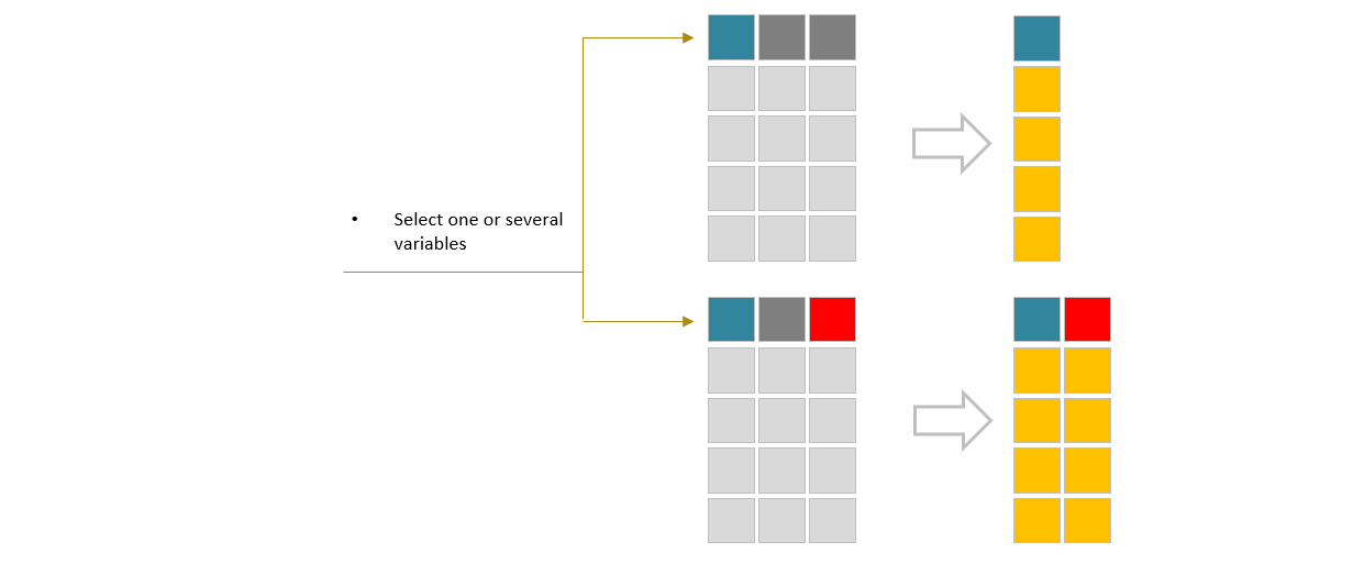
Let’s using the data frame Geo_data, and select only 2 variables : Cities and Population.
We can write the following syntax, using the |> operator, which means: “take the object [Geo_data] and then perform the action select() on it” (selection of only 2 variables: Cities and Population)
Geo_data |> select(Cities, Population) Cities Population
1 La Rochelle 74880
2 Saintes 25586
3 Rochefort 25183
4 Royan 17875
5 Aytre 8970
6 Tonnay-Charente 7739
7 Saint-Jean-d’Angely 7702
8 Perigny 7456
9 Angouleme 41740
10 Cognac 18825Can drop columns with -column
Using the function select() and adding a minus sign “-” before the name of a variable (or several variables), we can remove this variable from the data frame :
Geo_data |> select(-Departments) Cities Population
1 La Rochelle 74880
2 Saintes 25586
3 Rochefort 25183
4 Royan 17875
5 Aytre 8970
6 Tonnay-Charente 7739
7 Saint-Jean-d’Angely 7702
8 Perigny 7456
9 Angouleme 41740
10 Cognac 18825Reorder columns
We also can use the function select() to select the variables we need and display them in a particular order inside the data frame :
Geo_data |> select(Departments, Cities, Population) Departments Cities Population
1 Charente Maritime La Rochelle 74880
2 Charente Maritime Saintes 25586
3 Charente Maritime Rochefort 25183
4 Charente Maritime Royan 17875
5 Charente Maritime Aytre 8970
6 Charente Maritime Tonnay-Charente 7739
7 Charente Maritime Saint-Jean-d’Angely 7702
8 Charente Maritime Perigny 7456
9 Charente Angouleme 41740
10 Charente Cognac 18825everything()
Using the function everything(), we can bring a specific variable in the first or last position. Just need to type the name of the variable we want to relocate, and everything(), before or after it :
Geo_data |> select(Population, everything()) Population Cities Departments
1 74880 La Rochelle Charente Maritime
2 25586 Saintes Charente Maritime
3 25183 Rochefort Charente Maritime
4 17875 Royan Charente Maritime
5 8970 Aytre Charente Maritime
6 7739 Tonnay-Charente Charente Maritime
7 7702 Saint-Jean-d’Angely Charente Maritime
8 7456 Perigny Charente Maritime
9 41740 Angouleme Charente
10 18825 Cognac Charente10.2 add a variable
Let’s create a new variable (a column in the data frame) and perform a simple calculation. We use the approach we saw previously :
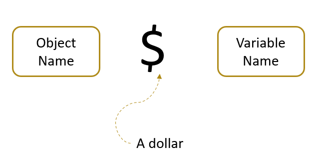
first, let’s create a clone, or copy, of the object Geo_data2 (so we don’t modify the initial data frame Geo_data2). We’ll call it “mycopy”. It’s an useful practice to keep some initial data.
then let’s create a new variable called “mynew_variable”.
this new variable is the result of a very simple calculation : we take the variable “Population” and multiply it by 100.
# create a copy of Geo_data2
mycopy <- Geo_data2

# create a variable, and perform a simple
mycopy$mynew_variable <- mycopy$Population*100

# display data frame
mycopy
Cities Population Departments mynew_variable
1 Bordeaux 254436 Gironde 25443600
2 Merignac 70105 Gironde 7010500
3 Pessac 63808 Gironde 6380800
4 Talence 42606 Gironde 4260600We can see that we now have a new variable, called “mynew_variable”, which is the result of the variable “Population”, multiplied by 100, for each row.
R performs operations by default along a variable (column) of a data frame.
Now, let’s add one new column with a character.
As previously, the same character value will be written along all the rows of the data frame.
# add one column Region
mycopy$Region <- "Nouvelle Aquitaine"

# display data frame
mycopy
Cities Population Departments mynew_variable Region
1 Bordeaux 254436 Gironde 25443600 Nouvelle Aquitaine
2 Merignac 70105 Gironde 7010500 Nouvelle Aquitaine
3 Pessac 63808 Gironde 6380800 Nouvelle Aquitaine
4 Talence 42606 Gironde 4260600 Nouvelle Aquitaine10.3 rbind() & cbind()
Very often, we need to combine several data frames into a single one, for example :
historical sales : historical sales data can be recorded for each month or year, inside distinct data frames.
inventories of different locations : stocks can be recorded separately in different warehouses (related to each country) or storage locations (duty free, duty paid,…).
etc…
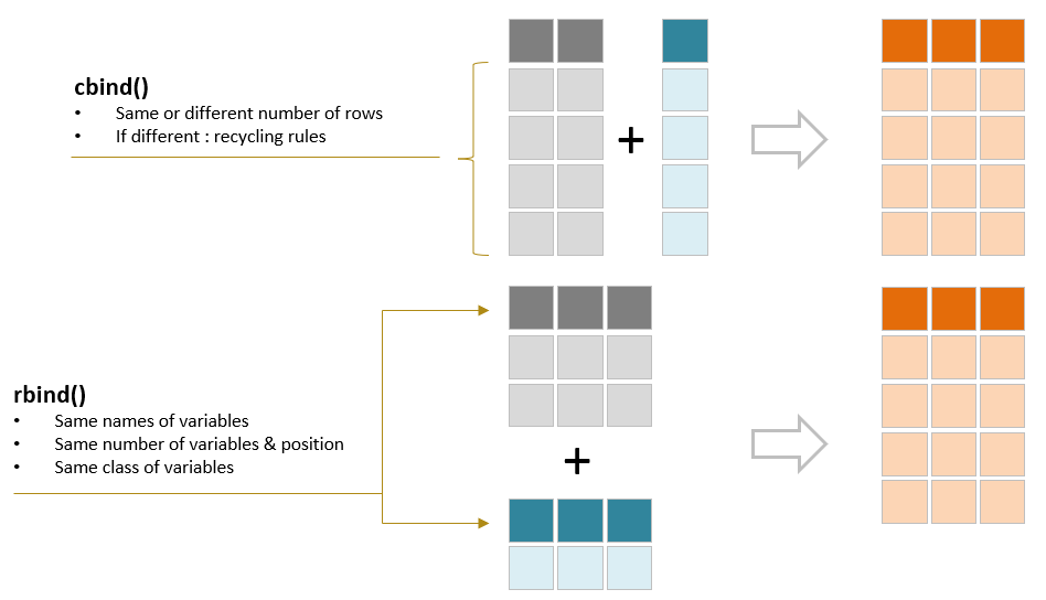
The functions rbind() and cbind() will allow us to easily combine -bind- some data frames together.
10.3.1 rbind()
The rbind() function allows to stack several data frames together.
One prerequisite, those data frames must have:
the same number of variables.
the same names of variables.
the same class of variables.
# combine 2 data frames
All_Geo_data <- rbind(Geo_data, Geo_data2)

# display data frame
All_Geo_data
Cities Population Departments
1 La Rochelle 74880 Charente Maritime
2 Saintes 25586 Charente Maritime
3 Rochefort 25183 Charente Maritime
4 Royan 17875 Charente Maritime
5 Aytre 8970 Charente Maritime
6 Tonnay-Charente 7739 Charente Maritime
7 Saint-Jean-d’Angely 7702 Charente Maritime
8 Perigny 7456 Charente Maritime
9 Angouleme 41740 Charente
10 Cognac 18825 Charente
11 Bordeaux 254436 Gironde
12 Merignac 70105 Gironde
13 Pessac 63808 Gironde
14 Talence 42606 Gironde10.3.2 cbind()
The cbind() function can be used to add one or several columns (i.e. a data frame) to one data frame.
In the following example example, we will “stick” the vector “Continent” to the data frame Geo_data2 :
# create a vector called "Continent"
Continent <- c("Europe","Europe","Europe","Europe")

# combine with Geo_data2
cbind(Geo_data2, Continent)
Cities Population Departments Continent
1 Bordeaux 254436 Gironde Europe
2 Merignac 70105 Gironde Europe
3 Pessac 63808 Gironde Europe
4 Talence 42606 Gironde Europelet’s explore the “recycling” feature
This vector “Continent” has 4 values. What happens if it had only 2 elements ?
This leads us to a sometimes very useful feature called “recycling”.
Let’s create a new vector “Continent” with only 2 elements this time, and bind it to the data frame Geo_data2.
We can see that the 2 elements are repeated on the following rows. This is the “recycling” feature.
# create a vector with just 2 elements
Continent <- c("Europe","To be confirmed")

# combine with Geo_data2
cbind(Geo_data2, Continent)
Cities Population Departments Continent
1 Bordeaux 254436 Gironde Europe
2 Merignac 70105 Gironde To be confirmed
3 Pessac 63808 Gironde Europe
4 Talence 42606 Gironde To be confirmed10.4 arrange()
The arrange() function allows us to sort a data frame based on one or several variables.
Let’s practice on the data frame All_Geo_data.
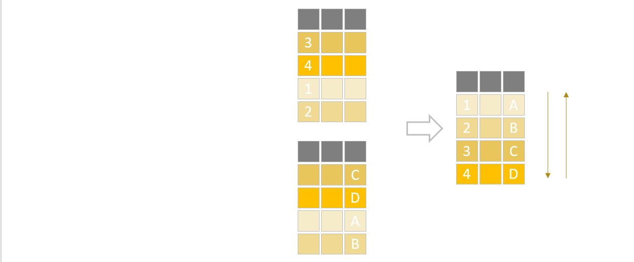
sort by ascending order
In the 2 examples below, we will sort from the beginning to the end :
by alphabetical order
by numerical values
By alphabetical order :
All_Geo_data |> arrange(Cities) Cities Population Departments
1 Angouleme 41740 Charente
2 Aytre 8970 Charente Maritime
3 Bordeaux 254436 Gironde
4 Cognac 18825 Charente
5 La Rochelle 74880 Charente Maritime
6 Merignac 70105 Gironde
7 Perigny 7456 Charente Maritime
8 Pessac 63808 Gironde
9 Rochefort 25183 Charente Maritime
10 Royan 17875 Charente Maritime
11 Saint-Jean-d’Angely 7702 Charente Maritime
12 Saintes 25586 Charente Maritime
13 Talence 42606 Gironde
14 Tonnay-Charente 7739 Charente MaritimeBy numerical values :
All_Geo_data |> arrange(Population) Cities Population Departments
1 Perigny 7456 Charente Maritime
2 Saint-Jean-d’Angely 7702 Charente Maritime
3 Tonnay-Charente 7739 Charente Maritime
4 Aytre 8970 Charente Maritime
5 Royan 17875 Charente Maritime
6 Cognac 18825 Charente
7 Rochefort 25183 Charente Maritime
8 Saintes 25586 Charente Maritime
9 Angouleme 41740 Charente
10 Talence 42606 Gironde
11 Pessac 63808 Gironde
12 Merignac 70105 Gironde
13 La Rochelle 74880 Charente Maritime
14 Bordeaux 254436 Girondesort by descending order
We can add and use the function desc() to sort by descending order, as follow :
All_Geo_data |> arrange(desc(Population)) Cities Population Departments
1 Bordeaux 254436 Gironde
2 La Rochelle 74880 Charente Maritime
3 Merignac 70105 Gironde
4 Pessac 63808 Gironde
5 Talence 42606 Gironde
6 Angouleme 41740 Charente
7 Saintes 25586 Charente Maritime
8 Rochefort 25183 Charente Maritime
9 Cognac 18825 Charente
10 Royan 17875 Charente Maritime
11 Aytre 8970 Charente Maritime
12 Tonnay-Charente 7739 Charente Maritime
13 Saint-Jean-d’Angely 7702 Charente Maritime
14 Perigny 7456 Charente Maritimesort by multiple variables
Now we are going to execute one after each other 2 different sortings :
first : sort by ascending Departments.
second : inside each Department, sort by descending Population.
The syntax is as follow :
All_Geo_data |> arrange(Departments,
                      desc(Population)
                      )
Cities Population Departments
1 Angouleme 41740 Charente
2 Cognac 18825 Charente
3 La Rochelle 74880 Charente Maritime
4 Saintes 25586 Charente Maritime
5 Rochefort 25183 Charente Maritime
6 Royan 17875 Charente Maritime
7 Aytre 8970 Charente Maritime
8 Tonnay-Charente 7739 Charente Maritime
9 Saint-Jean-d’Angely 7702 Charente Maritime
10 Perigny 7456 Charente Maritime
11 Bordeaux 254436 Gironde
12 Merignac 70105 Gironde
13 Pessac 63808 Gironde
14 Talence 42606 GirondeWe start by writing within the function arrange() the variable “Departments” and then the variable “Population”, itself within the function desc().
10.5 filter()
We can filter a data frame based on :
a variable.
multiple variables.
one or several values within those variables.
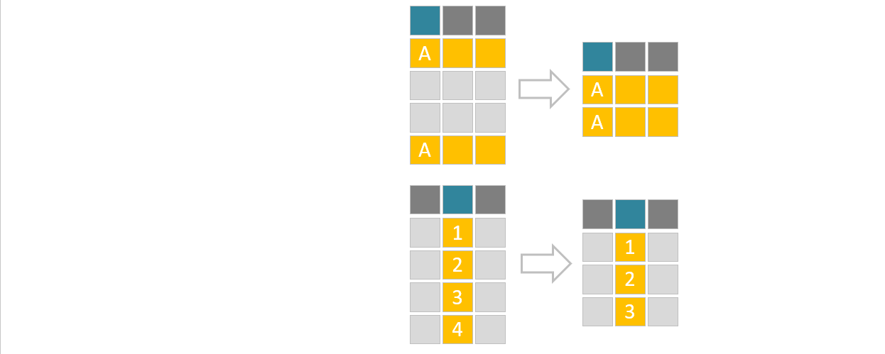
Filter : test for equality or multiple values
The function filter() keeps or discards rows (i.e observations) based on one or several values.
the
==operator tests for equality, referring to a single value (note that it comes with 2 signs =).the
%in%operator filters on several values. Those values are contain inside a vector.
Let’s practice on the data frame All_Geo_data :
# filter on Departments = Gironde
All_Geo_data |> filter(Departments == "Gironde")
Cities Population Departments
1 Bordeaux 254436 Gironde
2 Merignac 70105 Gironde
3 Pessac 63808 Gironde
4 Talence 42606 GirondeNow let’s filter, to keep 2 departments, “Charente” and “Gironde”. We will write those 2 departments inside a vector, and use the %in% operator to say that we want to select several variables.
# filter on Departments Charente and Gironde
All_Geo_data |> filter(Departments %in% c("Charente","Gironde"))
Cities Population Departments
1 Angouleme 41740 Charente
2 Cognac 18825 Charente
3 Bordeaux 254436 Gironde
4 Merignac 70105 Gironde
5 Pessac 63808 Gironde
6 Talence 42606 GirondeFilter <= or a range, using both >= & <=
Now let’s filter to keep all the rows with a population below 10.000 inhabitants.
# filter on Population below 10000
All_Geo_data |> filter(Population <= 10000)
Cities Population Departments
1 Aytre 8970 Charente Maritime
2 Tonnay-Charente 7739 Charente Maritime
3 Saint-Jean-d’Angely 7702 Charente Maritime
4 Perigny 7456 Charente MaritimeWe also can filter to keep all the rows with a population between 10.000 and 50.000 inhabitants.
# filter on Population between 10000 & 50000
All_Geo_data |> filter(Population >= 10000 & Population <= 50000)
Cities Population Departments
1 Saintes 25586 Charente Maritime
2 Rochefort 25183 Charente Maritime
3 Royan 17875 Charente Maritime
4 Angouleme 41740 Charente
5 Cognac 18825 Charente
6 Talence 42606 GirondeFilter : the | operator means “or”
We can combine 2 filters, applied on 2 different variables. Here is an example using the “or” operator, displayed as “|”.
We keep all the rows with a population above 70.000 inhabitants, OR from the Department “Charente” (whatever is the population of those cities).
All_Geo_data |> filter(Departments == "Charente" | Population >= 70000) Cities Population Departments
1 La Rochelle 74880 Charente Maritime
2 Angouleme 41740 Charente
3 Cognac 18825 Charente
4 Bordeaux 254436 Gironde
5 Merignac 70105 GirondeFilter : the & operator
We keep all the rows with a population below 50.000 inhabitants, AND from the Departments “Charente” & “Gironde”.
All_Geo_data |> filter(Departments %in% c("Charente","Gironde") & Population <= 50000) Cities Population Departments
1 Angouleme 41740 Charente
2 Cognac 18825 Charente
3 Talence 42606 Girondeexclude value
We also can filter to exclude one or several values. In this case we will use the sign “!” before the variable that we want to filter.
In the example below, we want to exclude the rows which contain 2 cities (La Rochelle and Royan) in the data frame All_Geo_data .
All_Geo_data |> filter(!Cities %in% c("La Rochelle", "Royan")) Cities Population Departments
1 Saintes 25586 Charente Maritime
2 Rochefort 25183 Charente Maritime
3 Aytre 8970 Charente Maritime
4 Tonnay-Charente 7739 Charente Maritime
5 Saint-Jean-d’Angely 7702 Charente Maritime
6 Perigny 7456 Charente Maritime
7 Angouleme 41740 Charente
8 Cognac 18825 Charente
9 Bordeaux 254436 Gironde
10 Merignac 70105 Gironde
11 Pessac 63808 Gironde
12 Talence 42606 Gironde10.6 count()
The function count() tallies a data frame by certain variable(s).
It’s useful to get a summary of the number of occurrences of some values.
All_Geo_data |> count(Departments) Departments n
1 Charente 2
2 Charente Maritime 8
3 Gironde 410.7 unique()
During our data manipulations, we will often need to handle duplicated values.
Sometimes, we will want to keep only the unique rows of a data frame.
This can be done easily by applying the function unique() to a data frame. To illustrate it, let’s create a data frame called df.
It’s also the opportunity to introduce here the function rep(), which provides an easy way to replicate one value.
For example, instead on writing: a <- c("A","A","A","B","B","B","C","C")
we can write : a <- c(rep("A", 3), rep("B", 3), rep("C",2))
# create a dummy dataframe
a <- c(rep("A", 3), rep("B", 3), rep("C",2))
b <- c(1,1,2,4,4,4,2,2)

# combine into 1 dataframe
df <- data.frame(a,b)

# display data frame
df
a b
1 A 1
2 A 1
3 A 2
4 B 4
5 B 4
6 B 4
7 C 2
8 C 2We can notice that some rows appear several times :
A & 1 : 2 times.
B & 4 : 3 times.
C & 2 : 2 times.
Let’s keep only the unique rows within the whole data frame.
Applying the function unique() we will remove the duplicated values.
# another way to select the unique values
df1 <- unique(df)

# display data frame
df1
a b
1 A 1
3 A 2
4 B 4
7 C 210.8 str_sub()
Let’s explore the function str_sub() from the R package stringr. This is the equivalent of the 2 functions left and right in Excel.
We continue practicing on the data frame All_Geo_data :
Extract of the first 3 characters of the variable “Cities”.
- we specify that we start from the value number 1, and end at the value number 3.
Extract of the last 3 characters of the variable “Cities”.
we specify that we start from the last value number 1, and end at the value number 3.
putting a minus sign “-” before the values 1 and 3.
# Extract the first 3 characters
str_sub(All_Geo_data$Cities, 1, 3)
[1] "La " "Sai" "Roc" "Roy" "Ayt" "Ton" "Sai" "Per" "Ang" "Cog" "Bor" "Mer"
[13] "Pes" "Tal"# Extract the last 3 characters
str_sub(All_Geo_data$Cities, -3, -1) [1] "lle" "tes" "ort" "yan" "tre" "nte" "ely" "gny" "eme" "nac" "aux" "nac"
[13] "sac" "nce"10.9 if then else
Writing an “if then else” statement is relatively easy in R, we can use the function if_else().
The function if_else() comes with 3 arguments: condition, value if true, value if false.
In the example below, we are going to create 2 locations, South and North, based on the Department. We say that if the Department is “Gironde”, then the location is the South.
# let's create a copy of the dataframe
df1 <- All_Geo_data

# create the variable Location
df1$Location <- if_else(df1$Departments == "Gironde", "South", "North")

# display data frame
df1
Cities Population Departments Location
1 La Rochelle 74880 Charente Maritime North
2 Saintes 25586 Charente Maritime North
3 Rochefort 25183 Charente Maritime North
4 Royan 17875 Charente Maritime North
5 Aytre 8970 Charente Maritime North
6 Tonnay-Charente 7739 Charente Maritime North
7 Saint-Jean-d’Angely 7702 Charente Maritime North
8 Perigny 7456 Charente Maritime North
9 Angouleme 41740 Charente North
10 Cognac 18825 Charente North
11 Bordeaux 254436 Gironde South
12 Merignac 70105 Gironde South
13 Pessac 63808 Gironde South
14 Talence 42606 Gironde SouthHere is another example with if else. This time, let’s use the initial data frame Geo_data.
Based on the population of each city, we will define a variable called “myrange”, to identify whether there are a “lot of people” (i.e. if more than 30.000 inhabitants), or “not many”, if it’s not the case.
# let's create a copy of the dataframe
df1 <- Geo_data

# affect a range
df1$myrange <- if_else(df1$Population > 30000, "a lot of people", "not many")

# display data frame
df1
Cities Population Departments myrange
1 La Rochelle 74880 Charente Maritime a lot of people
2 Saintes 25586 Charente Maritime not many
3 Rochefort 25183 Charente Maritime not many
4 Royan 17875 Charente Maritime not many
5 Aytre 8970 Charente Maritime not many
6 Tonnay-Charente 7739 Charente Maritime not many
7 Saint-Jean-d’Angely 7702 Charente Maritime not many
8 Perigny 7456 Charente Maritime not many
9 Angouleme 41740 Charente a lot of people
10 Cognac 18825 Charente not manyWe can refine this variable “myrange” :
add one more range : if between 10.000 and 20.000 inhabitants, “it looks like a middle size city”.
otherwise, keep the previous value of “myrange”.
We can write the following syntax :
# Add a new range
df1$myrange <- if_else(df1$Population > 10000 & df1$Population <= 30000, "it looks like a middle size city", df1$myrange)

# display data frame
df1
Cities Population Departments
1 La Rochelle 74880 Charente Maritime
2 Saintes 25586 Charente Maritime
3 Rochefort 25183 Charente Maritime
4 Royan 17875 Charente Maritime
5 Aytre 8970 Charente Maritime
6 Tonnay-Charente 7739 Charente Maritime
7 Saint-Jean-d’Angely 7702 Charente Maritime
8 Perigny 7456 Charente Maritime
9 Angouleme 41740 Charente
10 Cognac 18825 Charente
myrange
1 a lot of people
2 it looks like a middle size city
3 it looks like a middle size city
4 it looks like a middle size city
5 not many
6 not many
7 not many
8 not many
9 a lot of people
10 it looks like a middle size cityWe kept the previous values in my range and added some new ones.
This could also be seen as simple way to “nest” some “if then else” statements, through different steps.
We will see in the next part that there are other functions, such as case_when() which allows to create different cases, based on a range of values.
10.10 gsub()
When we clean some data, we often need to replace some values. The function gsub() will help us to implement those changes
It works as follow : gsub(pattern, replacement, targeted variable)
Let’s apply it on the data frame Geo_data2 :
# Create a working df
df1 <- Geo_data2

# substituting the value Bordeaux by Paris using gsub()
df1$Cities <- gsub("Bordeaux", "Paris the capital",df1$Cities)

# display data frame
df1
Cities Population Departments
1 Paris the capital 254436 Gironde
2 Merignac 70105 Gironde
3 Pessac 63808 Gironde
4 Talence 42606 GirondeWe replaced the value “Bordeaux” by the group of words “Paris is the capital”.
11 10 Intermediate Transformations
11.1 mutate()
The fonction mutate() creates one or several new variables. The new variables come with a single “=” .
In the example below we just had one variable, and it’s somehow similar to the syntax : dataset$my.new.variable.
All_Geo_data |> mutate(Country = "France") Cities Population Departments Country
1 La Rochelle 74880 Charente Maritime France
2 Saintes 25586 Charente Maritime France
3 Rochefort 25183 Charente Maritime France
4 Royan 17875 Charente Maritime France
5 Aytre 8970 Charente Maritime France
6 Tonnay-Charente 7739 Charente Maritime France
7 Saint-Jean-d’Angely 7702 Charente Maritime France
8 Perigny 7456 Charente Maritime France
9 Angouleme 41740 Charente France
10 Cognac 18825 Charente France
11 Bordeaux 254436 Gironde France
12 Merignac 70105 Gironde France
13 Pessac 63808 Gironde France
14 Talence 42606 Gironde FranceBut we can add more actions (variables), for example :
All_Geo_data |> mutate(Country = "France",
                       Continent = "Europe")
Cities Population Departments Country Continent
1 La Rochelle 74880 Charente Maritime France Europe
2 Saintes 25586 Charente Maritime France Europe
3 Rochefort 25183 Charente Maritime France Europe
4 Royan 17875 Charente Maritime France Europe
5 Aytre 8970 Charente Maritime France Europe
6 Tonnay-Charente 7739 Charente Maritime France Europe
7 Saint-Jean-d’Angely 7702 Charente Maritime France Europe
8 Perigny 7456 Charente Maritime France Europe
9 Angouleme 41740 Charente France Europe
10 Cognac 18825 Charente France Europe
11 Bordeaux 254436 Gironde France Europe
12 Merignac 70105 Gironde France Europe
13 Pessac 63808 Gironde France Europe
14 Talence 42606 Gironde France EuropeIt’s also often used when we want to chain different operations.
In the example below :
first we use an “if then else” statement and create a new variable called “Location”.
then, we apply on this result the function
select()to keep only 2 variables, “Cities” and (the newly created) “Location”.
All_Geo_data |>
    mutate(Location = if_else(Departments == "Gironde", "South", "North")) |>
    select(Cities, Location)
Cities Location
1 La Rochelle North
2 Saintes North
3 Rochefort North
4 Royan North
5 Aytre North
6 Tonnay-Charente North
7 Saint-Jean-d’Angely North
8 Perigny North
9 Angouleme North
10 Cognac North
11 Bordeaux South
12 Merignac South
13 Pessac South
14 Talence South11.2 case_when()
We previously looked at the “if then else” statement.
When there are multiple cases, the function case_when() can make our analysis much easier !
In the example below, we will define 3 cases :
first case : some cities are called “regional capitals”.
second case : another group of cities is called “small towns”.
third case : another group of cities is called “very small towns”.
the other cities are captured in a group called “to be defined”.
We will create a new variable using the function mutate(), and use the function case_when() to define those different cases, in this new variable.
All_Geo_data |> mutate(city_group = case_when(
  Cities %in% c("La Rochelle", "Angouleme", "Bordeaux") ~ "regional capitals",
  Cities %in% c("Saintes", "Rochefort", "Cognac", "Pessac", "Merignac", "Talence") ~ "small towns",
  Cities %in% c("Royan", "Aytre", "Tonnay-Charente") ~ "very small towns",
  TRUE ~ "to be defined")
  )
Cities Population Departments city_group
1 La Rochelle 74880 Charente Maritime regional capitals
2 Saintes 25586 Charente Maritime small towns
3 Rochefort 25183 Charente Maritime small towns
4 Royan 17875 Charente Maritime very small towns
5 Aytre 8970 Charente Maritime very small towns
6 Tonnay-Charente 7739 Charente Maritime very small towns
7 Saint-Jean-d’Angely 7702 Charente Maritime to be defined
8 Perigny 7456 Charente Maritime to be defined
9 Angouleme 41740 Charente regional capitals
10 Cognac 18825 Charente small towns
11 Bordeaux 254436 Gironde regional capitals
12 Merignac 70105 Gironde small towns
13 Pessac 63808 Gironde small towns
14 Talence 42606 Gironde small towns11.3 group_by()
The function group_by() is perfect to compute new variables by group.
For example, we can use it to calculate the percentage of amount of a group, as displayed below, creating a new variable “perc” using mutate() :
All_Geo_data |> group_by(Departments) |>
  mutate(perc = Population / sum(Population)
         )
# A tibble: 14 × 4
# Groups: Departments [3]
Cities Population Departments perc
<chr> <dbl> <chr> <dbl>
1 La Rochelle 74880 Charente Maritime 0.427
2 Saintes 25586 Charente Maritime 0.146
3 Rochefort 25183 Charente Maritime 0.144
4 Royan 17875 Charente Maritime 0.102
5 Aytre 8970 Charente Maritime 0.0511
6 Tonnay-Charente 7739 Charente Maritime 0.0441
7 Saint-Jean-d’Angely 7702 Charente Maritime 0.0439
8 Perigny 7456 Charente Maritime 0.0425
9 Angouleme 41740 Charente 0.689
10 Cognac 18825 Charente 0.311
11 Bordeaux 254436 Gironde 0.590
12 Merignac 70105 Gironde 0.163
13 Pessac 63808 Gironde 0.148
14 Talence 42606 Gironde 0.0989We get the % of population that each city represents within one Department.
This is very convenient when we need to define some weights or ratios for example.
11.4 group_by() & summarise()
Here comes the equivalent (in much more powerful way!) of the famous pivot table in Excel.
The functions group_by() and summarise() are used together to aggregate data :
group_by()identifies the grouping variable(s).summarise()specifies the aggregation (i.e. the action or calculation to be performed).
The figure below illustrates the concept : we have a data frame with similar values within one dimension, and want to aggregate the values of another (or more) variable around this (or those) dimension.
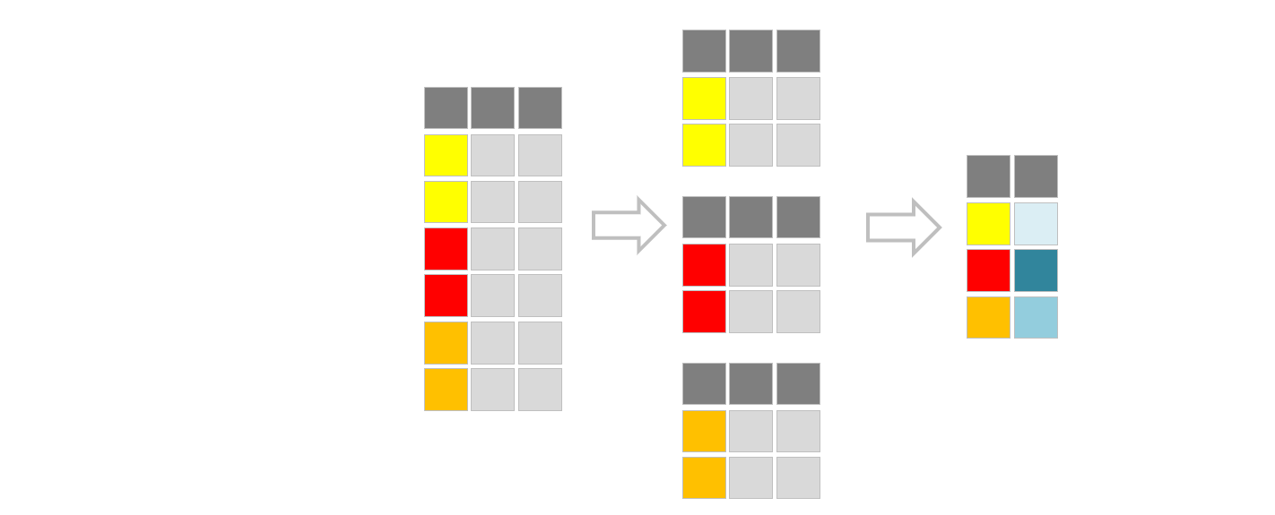
In the example below, we calculate the Total Population by Department, using the function sum() :
All_Geo_data |> group_by(Departments) |>
    summarise(total_population = sum(Population)
              )
# A tibble: 3 × 2
Departments total_population
<chr> <dbl>
1 Charente 60565
2 Charente Maritime 175391
3 Gironde 430955Other useful functions within summarise() are: mean(), median(), sd(), min(), max(), n(), n_distinct().
In the example below we calculate 2 new variables :
the Total Population by Department.
the number of cities (actually number of occurrences of rows) by Department, using the function
n().
All_Geo_data |> group_by(Departments) |>
    summarise(total_population = sum(Population),
              nb_cities = n()
              )
# A tibble: 3 × 3
Departments total_population nb_cities
<chr> <dbl> <int>
1 Charente 60565 2
2 Charente Maritime 175391 8
3 Gironde 430955 411.5 pivot
Data frames can be displayed in 2 ways : wide & long formats
During our data handling, we will need to pivot the data between those 2 formats. For this we can use from the R package tidyr :
the functions
spread()andgather().or also the functions
pivot_longer()andpivot_wider().
Those 2 pairs of functions work the same way.
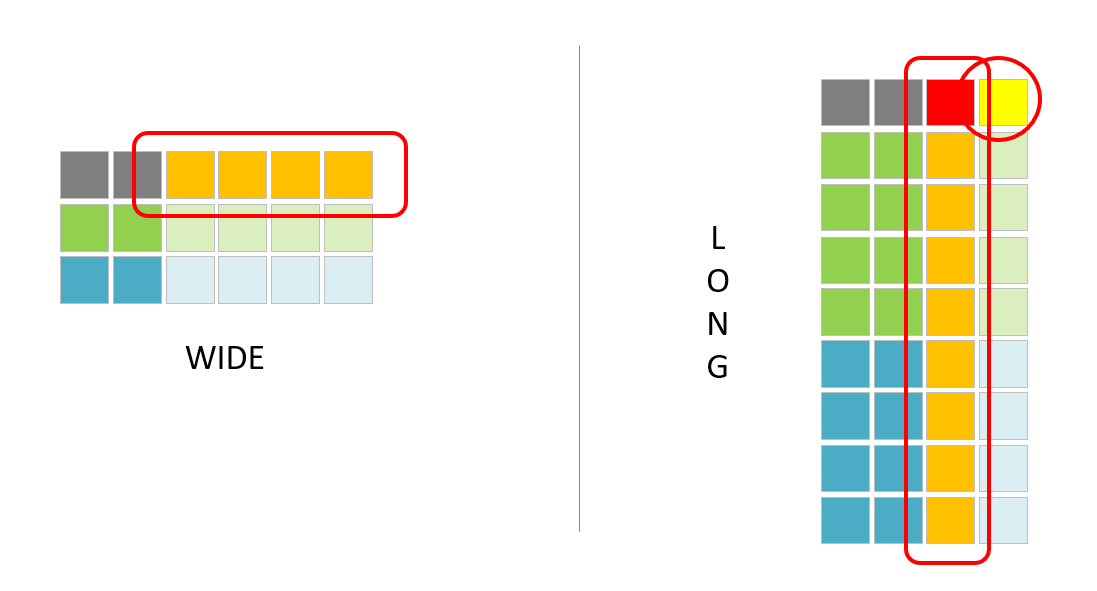
A wide format displays (spread) several columns (variables), which actually could also be gathered within a single common variable.
For example we can have a data frame in a wide format with different periods of time (January 2025, February 2025, …, December 2025). Those different periods of time could be gathered into one single variable called “period”, creating a longer (then less wide) data frame, as illustrated in the figure below :
Let’s create a demo data frame, in a long format.
# create vectors
products_family <- c(rep("Family 1", 8), rep("Family 2", 4))

products_description <- c(rep("Product A", 4), rep("Product B", 4), rep("Product C", 4))

period <- c(rep(c("2020/01/01", "2020/02/01", "2020/03/01", "2020/04/01"), 3))

sales <- c(10, 20, 30, 40,
           100, 200, 300, 400,
           5, 10, 15, 20
           )

# combine into one dataframe
initial_data <- data.frame(products_family,
                           products_description,
                           period,
                           sales)

# format the variable period as a date
initial_data$period <- as.Date(initial_data$period, format = "%Y/%m/%d")

# display data frame
initial_data
products_family products_description period sales
1 Family 1 Product A 2020-01-01 10
2 Family 1 Product A 2020-02-01 20
3 Family 1 Product A 2020-03-01 30
4 Family 1 Product A 2020-04-01 40
5 Family 1 Product B 2020-01-01 100
6 Family 1 Product B 2020-02-01 200
7 Family 1 Product B 2020-03-01 300
8 Family 1 Product B 2020-04-01 400
9 Family 2 Product C 2020-01-01 5
10 Family 2 Product C 2020-02-01 10
11 Family 2 Product C 2020-03-01 15
12 Family 2 Product C 2020-04-01 2011.5.1 transform to wide
We can apply the function spread(), to transform a long data frame into a wide one :
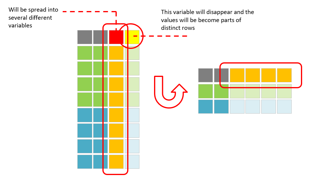
Let’s apply the function spread() on the data frame initial_data. We’re going to spread the variable “period” with its different unique values, into new variables :
# spread
df1 <- initial_data |> spread(period, sales)

# display data frame
df1
products_family products_description 2020-01-01 2020-02-01 2020-03-01
1 Family 1 Product A 10 20 30
2 Family 1 Product B 100 200 300
3 Family 2 Product C 5 10 15
2020-04-01
1 40
2 400
3 20We obtain a new data frame with the different periods of time in columns.
11.5.2 transform to long
To perform the opposite transformation, we can apply the function gather(). It transforms a wide data frame into a long one.
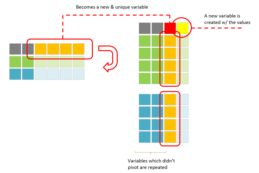
We keep the variables on the left, and we mention the names of the new ones that will be created after pivoting the data: 2 new variables will be created.
The function gather() comes with the function length().
The function length() counts the number of columns of a data frame i.e. its total length.
the “
:” means from x to y.in the example below, “:” means from the 3rd column until the last column.
Let’s first have a look at the function length() :
length(df1)[1] 6It returns the total number of variables of a data frame.
And now let’s apply the function gather() :
# apply gather
df1 <- df1 |> gather(key = "period",  # Name of the new key column
                     value = "sales", # Name of the new value column
                     3:length(df1)
                     )

# display data frame
df1
products_family products_description period sales
1 Family 1 Product A 2020-01-01 10
2 Family 1 Product B 2020-01-01 100
3 Family 2 Product C 2020-01-01 5
4 Family 1 Product A 2020-02-01 20
5 Family 1 Product B 2020-02-01 200
6 Family 2 Product C 2020-02-01 10
7 Family 1 Product A 2020-03-01 30
8 Family 1 Product B 2020-03-01 300
9 Family 2 Product C 2020-03-01 15
10 Family 1 Product A 2020-04-01 40
11 Family 1 Product B 2020-04-01 400
12 Family 2 Product C 2020-04-01 2011.6 joints
There are 4 types of joints : Left Join / Right Join / full join / natural join
The left join is the equivalent of a VLOOKUP in Excel. R provides broader (and easier) options to merge data frames compared to Excel, especially the capacity to perform a full join or a natural join operation.
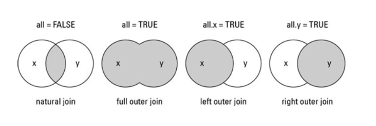
Let’s illustrate the different types of joints, merging 2 data frames.
We create a first data frame, with 2 variables : Cities and Countries
#----------------------------
# Create the 1st dataframe
#----------------------------

# create 2 vectors
Cities <- c("Shanghai","Tokyo","Sydney","Jakarta")
Countries <- c("China", "Japan", "Australia", "Indonesia")

# combine into 1 dataframe
Geo_data3 <- data.frame(Cities,Countries)

# display data frame
Geo_data3
Cities Countries
1 Shanghai China
2 Tokyo Japan
3 Sydney Australia
4 Jakarta IndonesiaAnd now a second data frame with 2 other variables : Countries and Regions
#----------------------------
# Create the 2nd dataframe
#----------------------------

# create 2 vectors
Countries <- c("South Korea","China", "New Zealand", "Japan", "Thailand", "Indonesia", "Malaysia", "Germany", "Brazil")

Regions <- c("APAC","APAC", "APAC", "APAC", "APAC", "APAC", "APAC", "EMEA", "LATAM")

# combine into 1 dataframe
Geo_data4 <- data.frame(Countries, Regions)

# display data frame
Geo_data4
Countries Regions
1 South Korea APAC
2 China APAC
3 New Zealand APAC
4 Japan APAC
5 Thailand APAC
6 Indonesia APAC
7 Malaysia APAC
8 Germany EMEA
9 Brazil LATAMThose 2 data frames have a common variable : Countries
Now, let’s illustrate the 4 types of joints.
11.6.1 left join
The function left_join() is the equivalent of the VLOOKUP in Excel :
we want to add the value of the variable “Regions” from the table on the right (i.e. Geo_data4) to the existing data frame Geo_data3 (i.e. table on the left).
since Australia is not present in the data frame Geo_data4, the Regions appears as “NA”.
# merge
Geo_data5 <- left_join(Geo_data3, Geo_data4)
Joining with `by = join_by(Countries)`# display data frame
Geo_data5 Cities Countries Regions
1 Shanghai China APAC
2 Tokyo Japan APAC
3 Sydney Australia <NA>
4 Jakarta Indonesia APAC11.6.2 right join
The function right_join() performs a similar operation with the previous one, but here we add to the table on the right (i.e. Geo_data4), the related elements of the table on the left (i.e. Geo_data3).
Only 3 Countries (China, Japan, Indonesia) are present in the data frame Geo_data3.
We then get the values of the Cities related to those Countries. For the other Countries, the values are missing and displayed as “NA”.
# merge
Geo_data6 <- right_join(Geo_data3, Geo_data4)
Joining with `by = join_by(Countries)`# display data frame
Geo_data6 Cities Countries Regions
1 Shanghai China APAC
2 Tokyo Japan APAC
3 Jakarta Indonesia APAC
4 <NA> South Korea APAC
5 <NA> New Zealand APAC
6 <NA> Thailand APAC
7 <NA> Malaysia APAC
8 <NA> Germany EMEA
9 <NA> Brazil LATAM11.6.3 natural join
This type of merge will keep only the rows that match from both data frames, i.e. the intersection between both.
We use the function merge() and specify the argument all = FALSE.
# merge
Geo_data7 <- merge(Geo_data3, Geo_data4, all = FALSE)

# display data frame
Geo_data7
Countries Cities Regions
1 China Shanghai APAC
2 Indonesia Jakarta APAC
3 Japan Tokyo APAC11.6.4 full outer join
This type of merge will keep all the rows from both data frames.
We use the function merge() and specify all = TRUE .
# Merge
Geo_data8 <- merge(Geo_data3, Geo_data4, all = TRUE)

# display data frame
Geo_data8
Countries Cities Regions
1 Australia Sydney <NA>
2 Brazil <NA> LATAM
3 China Shanghai APAC
4 Germany <NA> EMEA
5 Indonesia Jakarta APAC
6 Japan Tokyo APAC
7 Malaysia <NA> APAC
8 New Zealand <NA> APAC
9 South Korea <NA> APAC
10 Thailand <NA> APACWe fully merged the 2 data frames.
all the rows of each data frame are present.
the missing values appear as NA.
11.7 cross joint
A particular, and sometimes useful, type of joint is a cross joint. We can realize it using the function crossing() .
In the example below we have 2 data frames without any variables in common. However, we want to merge those 2 data frame. Using the function crossing() we can merge them and get as a result a new data frame with the values of the 2nd data frame repeated along each row of the 1st data frame.
# Example dataframes (reusing df1 and df2 from above)
df1 <- data.frame(code.article = c("A1", "A2", "A3"),
                  demand = c(100, 200, 300))

df2 <- data.frame(period = as.Date(c("2024-01-15", "2024-02-15", "2024-03-15")))

# Perform a cross join using tidyr's crossing function
combined_df <- tidyr::crossing(df1, df2)

# display data frame
combined_df
# A tibble: 9 × 3
code.article demand period
<chr> <dbl> <date>
1 A1 100 2024-01-15
2 A1 100 2024-02-15
3 A1 100 2024-03-15
4 A2 200 2024-01-15
5 A2 200 2024-02-15
6 A2 200 2024-03-15
7 A3 300 2024-01-15
8 A3 300 2024-02-15
9 A3 300 2024-03-1511.8 replace_na()
The previous data frame Geo_data8 has some missing values in the variable “Cities”.
We can replace all the rows with missing values in a variable using the function replace_na().
In the example below, we will replace the missing values (NA) by the value “to be defined”.
# set a working df
df1 <- Geo_data8

# replace NA
df1$Cities <- df1$Cities |> replace_na("to be defined")

# display data frame
df1
Countries Cities Regions
1 Australia Sydney <NA>
2 Brazil to be defined LATAM
3 China Shanghai APAC
4 Germany to be defined EMEA
5 Indonesia Jakarta APAC
6 Japan Tokyo APAC
7 Malaysia to be defined APAC
8 New Zealand to be defined APAC
9 South Korea to be defined APAC
10 Thailand to be defined APAC11.9 drop_na()
The previous data frame Geo_data8 has some missing values in the variable “Cities”. We can remove all the rows with missing values in this variable using the function drop_na() :
Geo_data8 |> drop_na(Cities) Countries Cities Regions
1 Australia Sydney <NA>
2 China Shanghai APAC
3 Indonesia Jakarta APAC
4 Japan Tokyo APAC11.10 Replace all missing values by zero
Let’s create the following data frame, with some missing values :
# Create a simple dataset
data <- data.frame(
  A = c(1, 2, NA, 4),
  B = c(NA, 2, 3, 4),
  C = c(1, NA, 3, 4)
)


# display data frame
data
A B C
1 1 NA 1
2 2 2 NA
3 NA 3 3
4 4 4 4Here are a 2 ways to replace all the NA :
# 1st way
data <- data |>
  mutate_all(replace_na, replace = 0)


# 2nd way : a very short one (maybe less “straightforward”)
data[is.na(data)] <- 0