# ETL
install.packages("tidyverse")
install.packages("sparkline")
install.packages("reshape2")
install.packages("DT")
install.packages("data.table")
install.packages("knitr")
install.packages("purrr")
install.packages("janitor")
install.packages("zoo")
install.packages("scales")
install.packages("writexl")
install.packages("htmltools")1 Get started with R
We’re going to code in R! Yahoooooooo…!
So…how to start ?
Where can we write our code, import some datasets, transform them and visualize some results ?
When we program in R there are (as per today, March 2026) 2 popular tools :
Both tools have been created by posit (formerly called RStudio), a leading company in data science.
Positron is a mix of RStudio and VS code, and will most probably replace RStudio in the future. As per today, both tools are available, and we will present how to use each of them, starting with RStudio and then moving to positron.
In this chapter, we are going to prepare our working environment to program in R.
It is structured into 4 parts :
Installation of R console and RStudio
Presentation of RStudio
Explanation of what is a Package
Installation of the main packages for our work
2 2 things you need to start working with R
To start programming in R you need 2 things :
the R console : this is the “engine” to process your code
an IDE (Integrated Development Editor) : either RStudio desktop or positron which provide a powerful user interface to code, with plenty of features
Both are open source and free.
2.1 Install R
You can download it from the CRAN website : https://cran.r-project.org/
The CRAN (Comprehensive R Archive Network) is the central, global network of servers that hosts and distributes the R programming language, its official documentation, and thousands of add-on packages that extend R’s functionality for statistical computing and data analysis, acting as the primary hub for R users to download and manage essential tools.
It serves as the main source for installing R itself (and manages all the updated versions) and its vast collection of packages (like dplyr, ggplot2, etc.).
2.2 Install RStudio
You can download the free RStudio desktop IDE from : https://posit.co/download/rstudio-desktop/
3 What is RStudio ?
RStudio is an IDE (Integrated Development Editor), which offers plenty of features to code in R (and also other languages), and especially allows us to easily :
create R documents
R script
quarto
visualize the objects, functions or values that we upload or create
visualize some results : charts, tables,…
manage the packages and libraries we want to use
run (execute) a script of code
There are much more features, for example to link RStudio to github, connect to a database, publish a document on quarto.org,…
The ones above are the functionalities that we will use the more often.
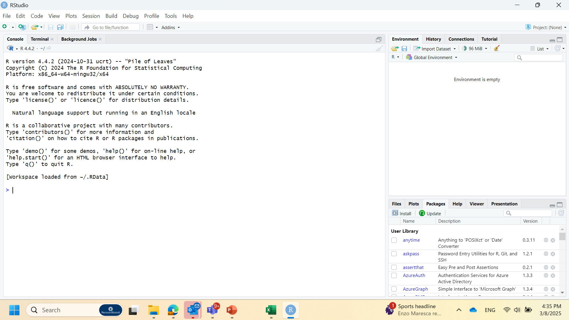
When we open RStudio, we can see 3 panels :
on the left side : a Console
we can write directly some code in it and execute it.
- but we cannot modify it and run it again; it’s a bit like a sand box.
when we run a R script or a quarto document, the code is executed (and displayed) line by line in the Console.
on the top right : the Environment
it’s where we will visualize the objects, functions or values that we upload or create.
there are 3 other tabs. To start (and keep it simple), we will essentially use the tab “Environment”.
on the bottom right :
there are 6 tabs. We will particularly use 2 : Packages and Plots.
in the tab “Packages” : we can see the different packages which are installed on our computer, and libraries we want to use.
in the tab “Plots” : we can visualize some results, for example a chart.
4 Create R documents
We will use 2 main types of documents :
a R Script
- it appears like a blank page, and will be used to create a function, or a Shiny web app for example.
a Quarto Document
it works like a notebook, with a table of contents.
to organize our data processing into different parts, a step also called ETL (Extract Transform Load)
to create some automated reports, including data visualization, and perform some analysis
To create a Quarto Document, go to File (on the top left of RStudio) => New File => Quarto Document
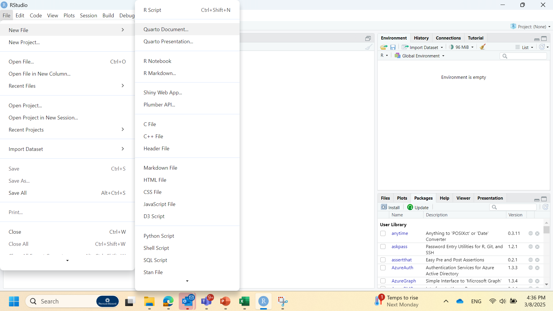
Very often in RStudio there are some shortcuts, here is another way, clicking on the icon “New File” on the top left :
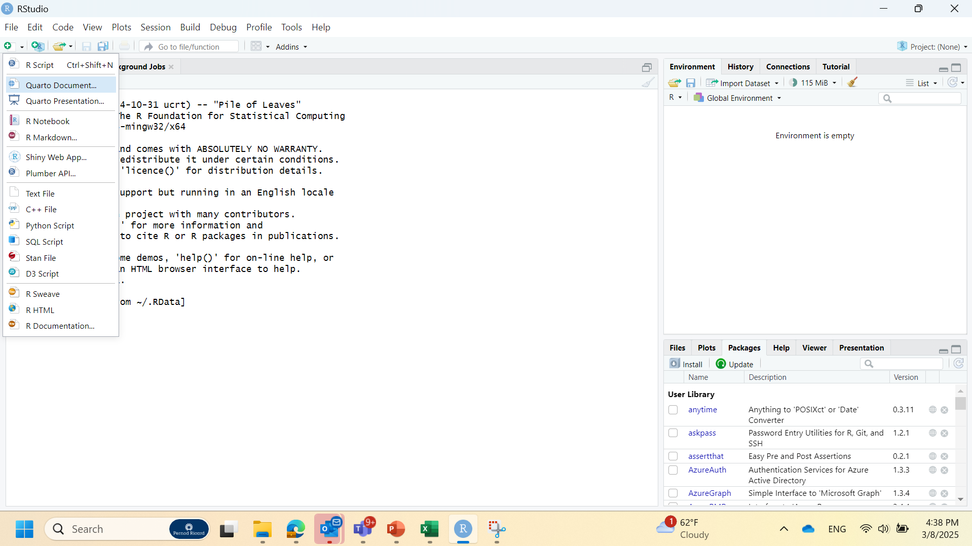
We also can create a R Script : go to File (on the top left of RStudio) => New File => R Script
As displayed below, with a blank page :
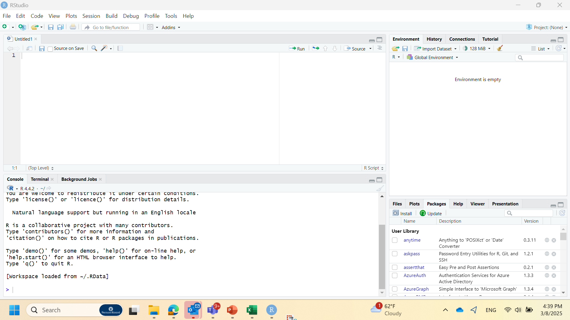
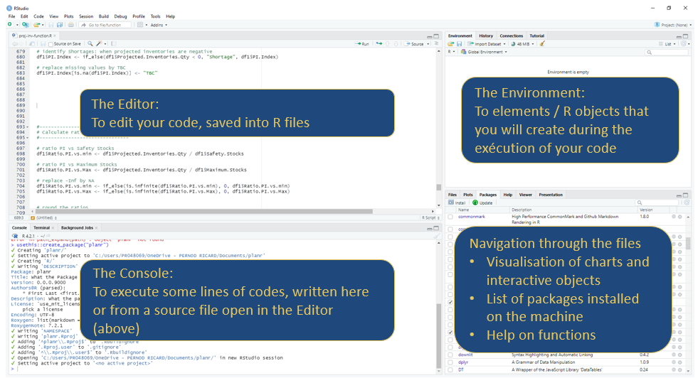
Once we have created a new document, whether it’s a R Script or a Quarto Document, we now have 4 panels in RStudio, as below :
the novelty here is the new panel on the top left.
it’s called “the Editor” : it’s where we will edit our code, and save the results into R files or qmd (quarto) files.
5 Packages
Before starting any new R project, we will always start by loading a few packages (or libraries) that we will use into our code.
A R Script or a Quarto Document will generally start with the packages that we will use later in the code.
5.1 What is a Package ?
R has a rich environment of Packages.
A Package is typically a collection of several codes in R (not necessarily written in R code!), which can be used to :
run some functions and perform some specific calculations, or create some visuals (charts, tables,…) :
tidyverse,highcharter,reactable,planrdevelop some web apps :
shiny,shinyWidgets,…connect to some external databases, create an API :
plumbr,AzureStor…
A package is a suitable way to organize our work and, if we want to, share it with others.
How To Install An R Package
A publicly available Package can be downloaded from 2 places : a github repository or the CRAN repository.
If we look at the R Package planr (Tools for Supply Chain Management, Demand and Supply Planning) , it’s available on :
The most common way is to use the CRAN repository: https://cran.r-project.org/
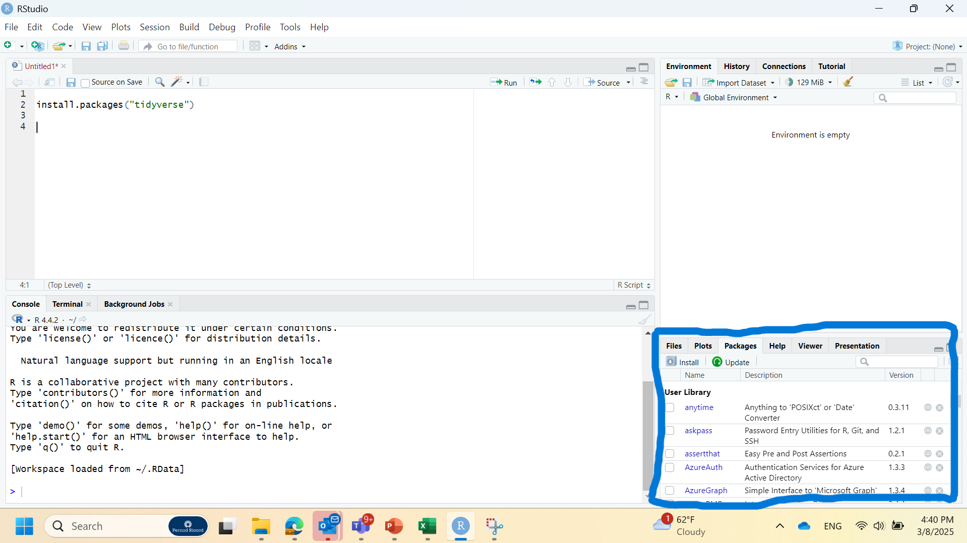
To install a package, you just need the name of the package and use the command install.packages("package").
As per today (March 2026), there are more than 23.000 packages available on CRAN.
Whether the Package is downloaded from github or from the CRAN, we only need to do this operation one time.
Then the Package will be downloaded and stored in your computer. It will also appear in the panel at the bottom right of RStudio.
5.2 Difference between a Package and a Library
In the context of R, the terms “package” and “library” are often used interchangeably, but they have distinct meanings:
R Package
A R package is a collection of R functions, data, and compiled code in a well-defined format.
It is a bundle of code, documentation, and tests that can be easily shared and reused.
Packages are created by developers and can be installed from repositories like CRAN (Comprehensive R Archive Network), Bioconductor, or GitHub.
Library
In R, the term “library” often refers to the function library() which is used to load an installed package into the current R session so that its functions and datasets can be used.
For example, when you run library(dplyr), you are loading the dplyr package so that its functions are available for use in your R session.
In summary, an R package is a collection of code and resources, while a library typically refers to the function used to load them into an R session.
6 Upload some key packages
Now, let’s configure our computer, and install a few essential packages that we will use through this book.
We only need to type this syntax install.packages("name of the package") one time. When we install a package, its name is written between 2 quotation marks.
Those packages will be for the ETL, data visualization (charts and tables), supply chain calculations, and to create interactive Shiny web apps.
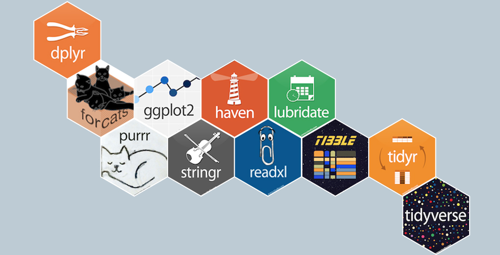
Note : a package is often built using other packages, so when we install one, we will also automatically install the other packages it uses. For example, as displayed in the Figure 9, the tidyverse package is a collection of several different packages (dplyr, lubridate,…)
6.1 for the ETL
6.2 for charts
# for Charts
install.packages("highcharter")
install.packages("RColorBrewer")
install.packages("plotly")
install.packages("leaflet")
install.packages("leaflet.extras")
install.packages("ggflowchart")
install.packages("DiagrammeR")
install.packages("d3Tree")
install.packages("collapsibleTree")
install.packages("networkD3")
6.3 for tables
# for Tables
install.packages("reactable")
install.packages("reactablefmtr")
install.packages("DT")
install.packages("rhandsontable")
install.packages("gtable")
install.packages("gtExtras")
install.packages("GWalkR")
6.4 for supply chain
Here we include packages related to forecasting and optimization, such as forecast and lpSolve, though their scope of application goes far beyond the supply chain.
# demand and supply planning
install.packages("planr")

# time series forecasting
install.packages("forecast")
install.packages("xgboost")
install.packages("timetk")
install.packages("caret")

# optimization
install.packages("lpSolve")
6.5 for shiny
# for Shiny
install.packages("shiny")
install.packages("shinythemes")
install.packages("shinyWidgets")
install.packages("shinydashboard")
install.packages("bslib")
7 How to activate a Package
After having installed one Package, we just need to load the Library to activate it in our session.
We can do this within a R Script or a Quarto Document, using the command library(name of the library) . When we load a Library, its name is not written between 2 quotation marks.
We also can notice that after running this command, the little box next to the name of the Package, at the the bottom right of RStudio, becomes ticked.
It means that the package is activated, and we can use the functions it contains.
Perfect ! Now we are ready to move on to the next step. In the next chapter we’re going to create a Quarto Document, to show how it works.