39  Using a BOM

As usual, we start by uploading the libraries that we’re going to use.

# ETL
library(tidyverse)

# Table
library(reactable)
library(reactablefmtr)

# Supply Chain
library(planr)

40 Context

We produce 3 Finished Goods A, B and C.

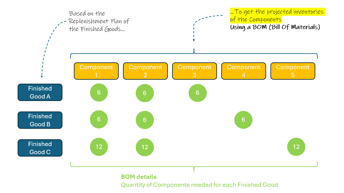
Those products have :

• some common components (components 1 and 2).

• some specific ones (components 3, 4 and 5).

We first calculate our Production Plan (through a DRP calculation) for the 3 Finished Goods, then, based on this, we will calculate the projected inventories on the 5 components.

To perform those calculations, we will use the R package planr.

Looking at the projected inventories on the components, we will be able to check if the calculated Production Plan is feasible considering the components’ current inventories, or if we have some supply constraints.

the objective here is to see how we can combine 2 different datasets to duplicate on purpose some rows, and use this feature for our BOM (Bill of Materials)

Figure 69 : BOM details

41 BOM (Bill Of Materials)

41.1 Original BOM (Matrix)

Let’s look at the BOM (Bill Of Materials) of the Finished Goods.

The Finished Good A is composed of :

• 6 elements of the Component 1.

• 6 elements of the Component 2.

• 6 elements of the Component 3.

The Finished Good B is composed of :

• 6 elements of the Component 1.

• 6 elements of the Component 2.

• 6 elements of the Component 4.

The Finished Good C follows the same logic, as represented in the table (data frame BOM_data) below, as a form of “matrix” :

#---------------
# Create BOM
#---------------

finished_good <- c("A", "B", "C")

component1 <- c(6, 6, 12)
component2 <- c(6, 6, 12)
component3 <- c(6, 0, 0)
component4 <- c(0, 6, 0)
component5 <- c(0, 0, 12)

BOM_data <- data.frame(finished_good,
                  component1,
                  component2,
                  component3,
                  component4,
                  component5)

#---------------
# display BOM
#---------------

BOM_data

  finished_good component1 component2 component3 component4 component5
1             A          6          6          6          0          0
2             B          6          6          0          6          0
3             C         12         12          0          0         12

41.2 Convert into flat BOM

To perform some calculations later on, it will be convenient to work with a “flat BOM”, that we will be able to combine easily with other data frames.

To create this flat BOM, we just need to pivot the data :

# set a working df
df1 <- BOM_data 

# pivot
df1 <- df1 |> gather(key = "component", 
                     value = "bom_qty", 
                     2:length(df1))

# keep results
flat_BOM_data <- df1

glimpse(df1)

Rows: 15
Columns: 3
$ finished_good <chr> "A", "B", "C", "A", "B", "C", "A", "B", "C", "A", "B", "…
$ component     <chr> "component1", "component1", "component1", "component2", …
$ bom_qty       <dbl> 6, 6, 12, 6, 6, 12, 6, 0, 0, 0, 6, 0, 0, 0, 12

42 Calculate DRP on Finished Goods

Now, let’s start by calculating a DRP (Distribution Requirement Planning, i.e. a Replenishment Plan) on the Finished Goods.

We just need a few variables :

• Demand Forecasts (monthly or weekly bucket).

• Opening Stocks on Hand (SoH).

• DRP parameters : safety stocks, frequency of supply,…

42.1 Create Template

Let’s upload a data frame with the monthly demand by Finished Goods.

We have 3 Finished Goods A, B and C, with their monthly demand forecasts.

We upload the 3 different variables (Demand Forecasts, Opening Stocks on Hand, DRP parameters) and combine them into a single data frame.

Demand

We upload the data frame from the github repository :

# Upload raw data

# Define the URL of the raw CSV file
url <- "https://raw.githubusercontent.com/nguyennico/bom_calculation/main/FG_Demand_data.csv"

# Read the CSV file from the URL
df1 <- read.csv(url)

# let's have a look at the dataset
head(df1)

  finished_good X7.1.2024 X8.1.2024 X9.1.2024 X10.1.2024 X11.1.2024 X12.1.2024
1             A        33        75       164         89         22        197
2             B        99       229       622        134        373       1720
3             C       262        75       785        168         93       1124
  X1.1.2025 X2.1.2025 X3.1.2025 X4.1.2025 X5.1.2025 X6.1.2025 X7.1.2025
1       348       176       284       220       252       330       255
2       682       343       551       419       486       275       612
3       403       202       325       252       289       309       580
  X8.1.2025 X9.1.2025 X10.1.2025 X11.1.2025 X12.1.2025 X1.1.2026 X2.1.2026
1       204       397        258        350        367       255       151
2       381      1183        621        842        760       587       346
3       396      1015        679        902        840       634       376
  X3.1.2026 X4.1.2026 X5.1.2026 X6.1.2026
1       197       216       181       211
2       372       562       435       572
3       527       554       411       453

And tidy it :

# Pivot
df1 <- df1 |> gather(key = "Period", 
                     value = "Demand", 
                     2:length(df1))

# remove the "X" in front of the period
df1$Period <- gsub("X", "", df1$Period)

# format date
df1$Period <- as.Date(as.character(df1$Period), format = '%m.%d.%Y')

# keep results
Demand_data <- df1

glimpse(df1)

Rows: 72
Columns: 3
$ finished_good <chr> "A", "B", "C", "A", "B", "C", "A", "B", "C", "A", "B", "…
$ Period        <date> 2024-07-01, 2024-07-01, 2024-07-01, 2024-08-01, 2024-08…
$ Demand        <int> 33, 99, 262, 75, 229, 75, 164, 622, 785, 89, 134, 168, 2…

Opening SoH

Now let’s create a data frame with the Opening Inventories, also called Opening SoH (Stocks On Hand).

# create vectors
finished_good <- c("A", "B", "C")

Opening <- c(400, 200, 500)

# combine
Opening_data <- data.frame(finished_good, Opening)

# add Period (beginning of the DRP horizon)
Opening_data$Period <- min(Demand_data$Period)

glimpse(Opening_data)

Rows: 3
Columns: 3
$ finished_good <chr> "A", "B", "C"
$ Opening       <dbl> 400, 200, 500
$ Period        <date> 2024-07-01, 2024-07-01, 2024-07-01

Assemble

As a last step, we :

• assemble the Demand, Opening SoH.

• add some DRP parameters (SSCocv, DRPCovDur, MOQ).

• define a Frozen Horizon (FH).

# merge
df1 <- left_join(Demand_data, Opening_data)

# replace missing values by zero
df1$Opening <- df1$Opening |> replace_na(0)

#---------------
# add other variables, needed to calculate a DRP
#---------------

# let's say there is no upcoming supply plan to consider
df1$Supply <- 0

# we set by default for all Finished Goods a safety stock of 2 months, and a replenishment frequency of every 2 months
df1$SSCov <- 2
df1$DRPCovDur <- 2

# other parameters
# we will start calculating the DRP from the very beginning : setting all the periods as "Free"
df1$MOQ <- 1
df1$FH <- "Free"



#---------------
# Final touch
#---------------

# rename
df1 <- df1 |> rename(DFU = finished_good)


# keep results
DRP_template_data <- df1

glimpse(df1)

Rows: 72
Columns: 9
$ DFU       <chr> "A", "B", "C", "A", "B", "C", "A", "B", "C", "A", "B", "C", …
$ Period    <date> 2024-07-01, 2024-07-01, 2024-07-01, 2024-08-01, 2024-08-01,…
$ Demand    <int> 33, 99, 262, 75, 229, 75, 164, 622, 785, 89, 134, 168, 22, 3…
$ Opening   <dbl> 400, 200, 500, 0, 0, 0, 0, 0, 0, 0, 0, 0, 0, 0, 0, 0, 0, 0, …
$ Supply    <dbl> 0, 0, 0, 0, 0, 0, 0, 0, 0, 0, 0, 0, 0, 0, 0, 0, 0, 0, 0, 0, …
$ SSCov     <dbl> 2, 2, 2, 2, 2, 2, 2, 2, 2, 2, 2, 2, 2, 2, 2, 2, 2, 2, 2, 2, …
$ DRPCovDur <dbl> 2, 2, 2, 2, 2, 2, 2, 2, 2, 2, 2, 2, 2, 2, 2, 2, 2, 2, 2, 2, …
$ MOQ       <dbl> 1, 1, 1, 1, 1, 1, 1, 1, 1, 1, 1, 1, 1, 1, 1, 1, 1, 1, 1, 1, …
$ FH        <chr> "Free", "Free", "Free", "Free", "Free", "Free", "Free", "Fre…

42.2 Calculate DRP

Our template is ready, and we can calculate the DRP, applying the function drp() from the package planr.

# set a working df
df1 <- DRP_template_data

# calculate drp
df1 <- planr::drp(data = df1,
                  DFU = DFU,
                  Period = Period,
                  Demand =  Demand,
                  Opening = Opening,
                  Supply = Supply,
                  SSCov = SSCov,
                  DRPCovDur = DRPCovDur,
                  MOQ = MOQ,
                  FH = FH)


# rename
df1 <- df1 |> rename(finished_good = DFU)

# keep results
FG_calculated_DRP_data <- df1

glimpse(df1)

Rows: 72
Columns: 15
$ finished_good                      <chr> "A", "A", "A", "A", "A", "A", "A", …
$ Period                             <date> 2024-07-01, 2024-08-01, 2024-09-01…
$ Demand                             <dbl> 33, 75, 164, 89, 22, 197, 348, 176,…
$ Opening                            <dbl> 400, 0, 0, 0, 0, 0, 0, 0, 0, 0, 0, …
$ Supply                             <dbl> 0, 0, 0, 0, 0, 0, 0, 0, 0, 0, 0, 0,…
$ SSCov                              <dbl> 2, 2, 2, 2, 2, 2, 2, 2, 2, 2, 2, 2,…
$ DRPCovDur                          <dbl> 2, 2, 2, 2, 2, 2, 2, 2, 2, 2, 2, 2,…
$ Stock.Max                          <dbl> 4, 4, 4, 4, 4, 4, 4, 4, 4, 4, 4, 4,…
$ MOQ                                <dbl> 1, 1, 1, 1, 1, 1, 1, 1, 1, 1, 1, 1,…
$ FH                                 <chr> "Free", "Free", "Free", "Free", "Fr…
$ Safety.Stocks                      <dbl> 239, 253, 111, 219, 545, 524, 460, …
$ Maximum.Stocks                     <dbl> 350, 472, 656, 743, 1005, 1028, 932…
$ DRP.Calculated.Coverage.in.Periods <dbl> 4.1, 3.1, 2.1, 4.0, 3.0, 4.0, 3.0, …
$ DRP.Projected.Inventories.Qty      <dbl> 367, 292, 128, 743, 721, 1028, 680,…
$ DRP.plan                           <dbl> 0, 0, 0, 704, 0, 504, 0, 582, 0, 45…

The variable DRP.plan stands for the (theoretical) Production Plan.

Now, we’re ready to combine the production plan of the finished goods with the flat BOM to calculate the related Demand on the Components.

43 Calculate Components Projected Inventories

43.1 Create Template

We need 3 components to calculate the projected inventories :

• Demand Forecasts : coming from the Finished Goods.

• Opening Inventories.

• Supply Plan :

  • that we will set here to zero; which means we don’t consider any coming supply plan. The idea is just to check how long can cover our current Stocks On Hand.

  • another scenario will be to consider an existing supply plan (and also to calculate a new one).

Demand

The Demand on the Components is the variable DRP.plan from the previous data frame.

We will :

• select this Demand (DRP.plan) as an input.

• merge this data frame with the flat BOM to calculate the related Demand on the Components.

Let’s note that when we realize this merger, we have a “many-to-many relationship”.

Concretely : a Finished Good A is present several times in the data frame of the flat BOM, so when we merge this data frame with the other one, it generates some additional rows.

It’s exactly what we aim to.

The result is a new data frame with for each period of time, the Demand (DRP.plan), the list of components of a Finished Good and their related bom_qty.

We’re then ready to calculate the related Demand on the components, by multiplying the DRP.plan by the bom_qty.

#---------------
# Get Demand from Finished Goods
#---------------

# set a working df
df1 <- FG_calculated_DRP_data

# keep only needed variables
df1 <- df1 |> select(finished_good, Period, DRP.plan)


#---------------
# Get Demand on Components
#---------------

# merge with flat BOM
df1 <- left_join(df1, flat_BOM_data)

Warning in left_join(df1, flat_BOM_data): Detected an unexpected many-to-many relationship between `x` and `y`.
ℹ Row 1 of `x` matches multiple rows in `y`.
ℹ Row 1 of `y` matches multiple rows in `x`.
ℹ If a many-to-many relationship is expected, set `relationship =
  "many-to-many"` to silence this warning.

# calculate the Demand on Compoments
df1$Demand <- df1$DRP.plan * df1$bom_qty

# replace missing values by zero
df1$Demand <- df1$Demand |> replace_na(0)

# aggregate
df1 <- df1 |> group_by(component, Period) |>
  summarise(Demand = sum(Demand)
            )

# keep results
Components_Demand_data <- df1

glimpse(df1)

Rows: 120
Columns: 3
Groups: component [5]
$ component <chr> "component1", "component1", "component1", "component1", "com…
$ Period    <date> 2024-07-01, 2024-08-01, 2024-09-01, 2024-10-01, 2024-11-01,…
$ Demand    <dbl> 18138, 0, 32736, 4224, 11688, 3024, 11922, 3492, 15990, 2754…

Opening SoH

Now let’s create a data frame with the Opening Inventories for the Components, as we previously did for the Finished Goods.

# create vectors
component <- c("component1",
               "component2",
               "component3",
               "component4",
               "component5")

Opening <- c(50000, 60000, 10000, 10000, 30000)

# combine
Components_Opening_data <- data.frame(component, Opening)

# add Period (beginning of the DRP horizon)
Components_Opening_data$Period <- min(Components_Demand_data$Period)

glimpse(Components_Opening_data)

Rows: 5
Columns: 3
$ component <chr> "component1", "component2", "component3", "component4", "com…
$ Opening   <dbl> 50000, 60000, 10000, 10000, 30000
$ Period    <date> 2024-07-01, 2024-07-01, 2024-07-01, 2024-07-01, 2024-07-01

Assemble

And as a last step, let’s assemble.

Here we simply want to look at the projected inventories and see whether with the current Stocks on Hand we have enough stocks to cover the Demand, then we will consider the Components’ Supply as zero.

Let’s note that in the reality we might have a current Supply Plan to be considered.

# merge
df1 <- left_join(Components_Demand_data, Components_Opening_data)

# replace missing values by zero
df1$Opening <- df1$Opening |> replace_na(0)

#---------------
# add other variables
#---------------

# let's say there is no upcoming supply plan to consider
df1$Supply <- 0


#---------------
# Final touch
#---------------

# rename
df1 <- df1 |> rename(DFU = component)


# keep results
PI_template_data <- df1

glimpse(df1)

Rows: 120
Columns: 5
Groups: DFU [5]
$ DFU     <chr> "component1", "component1", "component1", "component1", "compo…
$ Period  <date> 2024-07-01, 2024-08-01, 2024-09-01, 2024-10-01, 2024-11-01, 2…
$ Demand  <dbl> 18138, 0, 32736, 4224, 11688, 3024, 11922, 3492, 15990, 2754, …
$ Opening <dbl> 50000, 0, 0, 0, 0, 0, 0, 0, 0, 0, 0, 0, 0, 0, 0, 0, 0, 0, 0, 0…
$ Supply  <dbl> 0, 0, 0, 0, 0, 0, 0, 0, 0, 0, 0, 0, 0, 0, 0, 0, 0, 0, 0, 0, 0,…

43.2 Calculate Projected Inventories

Now we’re good to calculate the Components’ projected inventories, using the function light_proj_inv() from the R package planr.

# set a working df
df1 <- PI_template_data

# calculate
df1 <- planr::light_proj_inv(dataset = df1, 
                             DFU = DFU, 
                             Period = Period, 
                             Demand =  Demand, 
                             Opening = Opening, 
                             Supply = Supply)

# keep results
Calculated_PI_Components_data <- df1

glimpse(df1)

Rows: 120
Columns: 7
$ DFU                            <chr> "component1", "component1", "component1…
$ Period                         <date> 2024-07-01, 2024-08-01, 2024-09-01, 20…
$ Demand                         <dbl> 18138, 0, 32736, 4224, 11688, 3024, 119…
$ Opening                        <dbl> 50000, 0, 0, 0, 0, 0, 0, 0, 0, 0, 0, 0,…
$ Calculated.Coverage.in.Periods <dbl> 2.0, 1.0, 0.0, 0.0, 0.0, 0.0, 0.0, 0.0,…
$ Projected.Inventories.Qty      <dbl> 31862, 31862, -874, -5098, -16786, -198…
$ Supply                         <dbl> 0, 0, 0, 0, 0, 0, 0, 0, 0, 0, 0, 0, 0, …

Et voila!

43.3 Display Projected Inventories

Let’s look at the “component 3” and display the projected inventories, using the R packages reactable and reactablefmtr.

As we previously saw, it’s a 4 steps approach : Get data => Filter => Transform => Display (table or chart).

We can see that the current Opening Inventories are enough to cover the Finished Goods demand until February 2025.

#-------------------
# Get data
#-------------------

# set a working df
df1 <- Calculated_PI_Components_data


#-------------------
# Filter
#-------------------

# select component
df1 <- df1 |> filter(DFU == "component3")

#-------------------
# Transform
#-------------------

# keep only the needed columns
df1 <- df1 |> select(Period,
                     Demand,
                     Calculated.Coverage.in.Periods,
                     Projected.Inventories.Qty,
                     Supply)


# create a f_colorpal field
df1 <- df1 |> mutate(f_colorpal = case_when( 
  Calculated.Coverage.in.Periods > 6 ~ "#FFA500",
  Calculated.Coverage.in.Periods > 2 ~ "#32CD32",
  Calculated.Coverage.in.Periods > 0 ~ "#FFFF99",
  TRUE ~ "#FF0000" ))



#-------------------
# Table
#-------------------


# create reactable
reactable(df1, 
          resizable = TRUE, 
          showPageSizeOptions = TRUE,
          striped = TRUE, highlight = TRUE, compact = TRUE,
          defaultPageSize = 20,
          
          
          columns = list(
            
            Demand = colDef(
              name = "Demand (units)",
              cell = data_bars(df1,
                               fill_color = "#3fc1c9",
                               text_position = "outside-end")
              ),
            
            Calculated.Coverage.in.Periods = colDef(
              name = "Coverage (Periods)",
              maxWidth = 90,
              cell= color_tiles(df1, color_ref = "f_colorpal")
              ),
            
            f_colorpal = colDef(show = FALSE), # hidden, just used for the coverages
            
            Projected.Inventories.Qty = colDef(
              name = "Projected Inventories (units)",
              format = colFormat(separators = TRUE, digits=0),
              
              style = function(value) {
                if (value > 0) {
                  color <- "#008000"
                  } else if (value < 0) {
                    color <- "#e00000"
                    } else {
                      color <- "#777"
                      }
                list(color = color)
                }
              ),
            
            
            Supply = colDef(
              name = "Supply (units)",
              cell = data_bars(df1,
                               fill_color = "#3CB371",
                               text_position = "outside-end")
              )
            
            
            ), # close columns list
          
          
          columnGroups = list(
            
            
            colGroup(name = "Projected Inventories", 
                     columns = c("Calculated.Coverage.in.Periods",
                                 "Projected.Inventories.Qty"))
            
            ) # close columnGroups list
          
          
          ) # close reactable