# ETL
library(tidyverse)
library(reshape2)
library(sparkline)

# Charts
library(highcharter)

# Table
library(reactable)
library(reactablefmtr)

# Others
library(htmltools)47 RFM analysis
48 Context
We sell a product to more than 1000 stores.
In Demand Planning, we often aggregate all the historical sales to calculate some statistical forecasts for a product (this could be done at a country level, or at a channel level for example). However, in order to well understand the dynamic of the sales, and to see whether the statistical forecasts are relevant, it is also useful to look at the sales by customers.
If there are many customers, looking at the evolution of the sales for each outlet can be quite difficult to analyze, especially if each customer represents a tiny percentage of the total sales.
Therefore, a very simple and insightful approach is to perform a RFM (Recency, Frequency, Monetary) analysis, aiming to look at the historical purchases of each customer, and to group them into some segments, as described below.
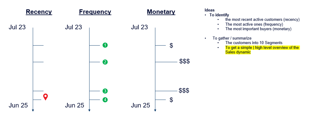
The RFM analysis is based on 3 axes :
Recency : did the customer buy recently?
Frequency : how often does the customer buy?
Monetary : does the customer buy a lot?
It informs us quickly about the sales dynamic :
are we gaining some new customers?
are we losing some customers?
what is the impact of the customers that we gain or loose?
how do our main (“champions”) customers evolve?
If we don’t have the Monetary in sales amount, it’s also fine to use the volumes as a first approach, especially if the selling price is the same for each customer.
The picture below summarizes the RFM concept :
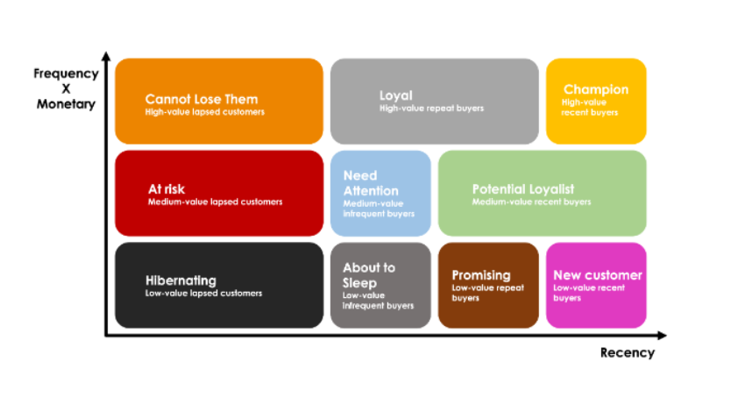
The traditional approach is to define 10 segments to group our customers.
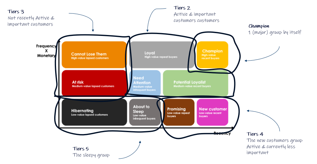
However, this sometimes can look a bit too detailed, and we also can have a higher hierarchy, to reduce the number of groups. For example, we can define 5 Higher level groups (of segments) as described in the figure 3.
Now, let’s see how to perform the RFM analysis on a simple dataset.
Upload libraries
49 Overview demo dataset
49.1 Get data
Let’s download a demo dataset from the GitHub repository below.
It’s a data frame with 7 variables :
a product.
a period of time.
some outlets numbers.
some dates features :
calendar_month_abb.
fiscal_year.
fiscal_month.
# Upload dataset

# Define the URL of the raw CSV file
url <- "https://raw.githubusercontent.com/nguyennico/rfm_analysis_practice/main/rfm_sales_data.csv"

# Read the CSV file from the URL
df1 <- read.csv(url)

# format period
df1$period <- as.Date(df1$period, format = "%m/%d/%Y")

# Get Calendar.Month
df1$calendar_month <- month(df1$period)

# Add Calendar.Month.abb
df1$calendar_month_abb <- month.abb[df1$calendar_month]


#-----------------------
# Add fiscal_year
#-----------------------

df1$fiscal_year <- if_else(df1$period >= "2023-07-01" & df1$period <= "2024-06-01",
                           "FY24", "TBC")

df1$fiscal_year <- if_else(df1$period >= "2024-07-01" & df1$period <= "2025-06-01",
                           "FY25", df1$fiscal_year)


#----------------------
# Add fiscal_month
# Create Fiscal_Calendar_DB
#----------------------

calendar_month <- c(7:12, 1:6)
fiscal_month <- c(1:12)

# Create a Fiscal Calendar
Fiscal_Calendar_data <- data.frame(calendar_month,
                                    fiscal_month)


#----------------------
# Merge
#----------------------

df1 <- left_join(df1, Fiscal_Calendar_data)

# remove not needed variables
df1 <- df1 |> select(-calendar_month)

# create a factor
df1$calendar_month_abb <- factor(df1$calendar_month_abb,
                                 levels = c("Jul","Aug","Sep","Oct","Nov","Dec",
                                 "Jan","Feb","Mar","Apr","May","Jun"))

# keep results
rfm_sales_data <- df1

glimpse(df1)
Rows: 6,994
Columns: 7
$ product <chr> "item1", "item1", "item1", "item1", "item1", "item1…
$ period <date> 2023-07-01, 2023-08-01, 2023-09-01, 2023-12-01, 20…
$ outlet_no <chr> "outlet1", "outlet1", "outlet1", "outlet1", "outlet…
$ sales_qty <dbl> 1.8667, 4.2000, 20.5334, 6.0667, 0.4667, 2.8000, 5.…
$ calendar_month_abb <fct> Jul, Aug, Sep, Dec, Feb, Mar, Sep, Jan, Jun, Aug, D…
$ fiscal_year <chr> "FY24", "FY24", "FY24", "FY24", "FY24", "FY24", "FY…
$ fiscal_month <int> 1, 2, 3, 6, 8, 9, 3, 7, 12, 2, 6, 2, 3, 4, 5, 6, 7,…49.2 Overview
Let’s get an overview, creating a summary table with the sales per outlet and per fiscal year.
The idea is to visualize the number of outlets, the evolution of their sales and the share of the total volume that they represent.
# set a working df
df1 <- rfm_sales_data

# aggregate
df1 <- df1 |> group_by(outlet_no, fiscal_year) |>
  summarise(sales_qty = sum(sales_qty)
            )

# spread
df1 <- df1 |> spread(fiscal_year, sales_qty)

# formatting
df1 <- as.data.frame(df1)

# replace missing values by zero
df1$FY24 <- df1$FY24 |> replace_na(0)
df1$FY25 <- df1$FY25 |> replace_na(0)

# calculate % of total FY25 sales
df1$FY25_pc <- df1$FY25 / sum(df1$FY25)


# calculate differences
df1$delta_value <- df1$FY25 - df1$FY24
df1$delta_value_pc <- df1$delta_value / df1$FY24


# replace -inf by zero
df1$delta_value_pc <- if_else(is.infinite(df1$delta_value_pc),
                              0,
                              df1$delta_value_pc)


# replace missing by zero
df1$delta_value_pc <- if_else(is.na(df1$delta_value_pc),
                              0,
                              df1$delta_value_pc)


# sort by descending FY25 amount
df1 <- df1 |> arrange(desc(FY25))

# calculate the accumulated % of FY25 amount that each outlet represents
df1$acc_FY25_pc <- cumsum(df1$FY25_pc)


# keep results
fiscal_year_summary_data <- df1

head(fiscal_year_summary_data)
outlet_no FY24 FY25 FY25_pc delta_value delta_value_pc acc_FY25_pc
1 outlet844 156.3336 323.3999 0.03871861 167.0663 1.0686525 0.03871861
2 outlet282 134.4000 283.7336 0.03396962 149.3336 1.1111131 0.07268823
3 outlet36 157.5002 176.3999 0.02111924 18.8997 0.1199979 0.09380747
4 outlet368 33.9109 155.4000 0.01860505 121.4891 3.5825973 0.11241252
5 outlet177 44.4113 146.2221 0.01750624 101.8108 2.2924526 0.12991876
6 outlet88 81.0446 127.0888 0.01521553 46.0442 0.5681341 0.14513429We can see that :
we have more than 1000 outlets.
the TOP 20 outlets represent 30% of the total FY25 sales amount, and the TOP 145 represent 80% of the sales, quite close to the Pareto distribution (20% of the outlets represent about 80% of the sales).
the comparison between FY25 and FY24 shows some high variations for some outlets.
Let’s apply the RFM analysis to get a more compact overview, and understand the dynamic of the outlets, by gathering them into some segments.
50 RFM analysis
50.1 Calculate RFM
Let’s calculate the Recency, Frequency, and Monetary values for each customer.
We define a variable analysis_date to set the last date of the records, from which we will calculate the Recency value.
# set a working df
df1 <- rfm_sales_data

# define the date of analysis
analysis_date <- "2025-06-01" #here, the last date of our dataset

# Recency: Days since last purchase
recency_df <- df1 |>
      group_by(outlet_no) |>
      summarise(LastPurchaseDate = max(period)) |>
      mutate(Recency = as.numeric(difftime(analysis_date,
                                           LastPurchaseDate,
                                           units = "days")))


# Frequency: Number of purchases
frequency_df <- df1 |>
      group_by(outlet_no) |>
      summarise(Frequency = n())


# Monetary: Total sales amount
monetary_df <- df1 |>
      group_by(outlet_no) |>
      summarise(Monetary = sum(sales_qty))


# Combine RFM values into one dataframe
rfm_df <- recency_df |>
      inner_join(frequency_df, by = "outlet_no") |>
      inner_join(monetary_df, by = "outlet_no")


glimpse(rfm_df)
Rows: 1,054
Columns: 5
$ outlet_no <chr> "outlet1", "outlet10", "outlet100", "outlet1000", "ou…
$ LastPurchaseDate <date> 2024-09-01, 2023-10-01, 2025-06-01, 2024-06-01, 2025…
$ Recency <dbl> 272.6666667, 608.6666667, -0.3333333, 364.6666667, -0…
$ Frequency <int> 7, 1, 19, 5, 3, 1, 3, 3, 7, 8, 11, 1, 1, 15, 1, 3, 1,…
$ Monetary <dbl> 41.9224, 0.4667, 20.1450, 21.1556, 6.8445, 0.2333, 1.…50.2 Assign RFM scores
Now, let’s assign some scores to each outlets.
For this, we will rank and separate each outlet based on the distribution of their values.
we create 4 groups of quartile : 0 to 25%, 25% to 50%, 50% to 75%.
and affect values to groups for each variable (Recency | Frequency | Monetary).
We will rank the outlets’ values by ascending order, and then create 4 groups of quartile, as below :
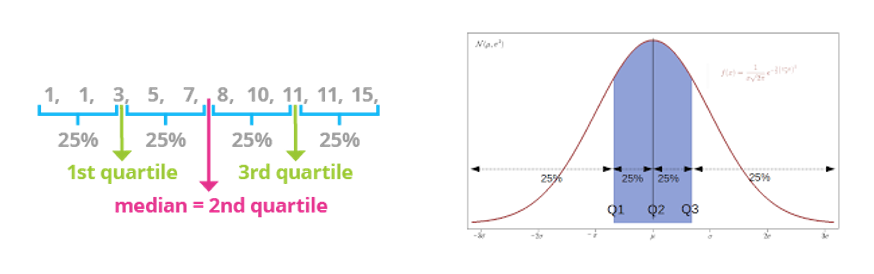
Following this methodology, we’re going to calculate 3 groups : for the Recency, the Frequency and the Monetary.
We will use the functions cut() and quantile() . Those 2 functions are available as base of the R package, requiring no external packages.
The
cut()function is used to divide a continuous numeric vector into intervals (or “bins”) and convert it into a categorical factor.The basic syntax is
cut(x, breaks, labels, include.lowest, right).x: the numeric vector to be divided.
breaks: can be a numeric vector of cut points or a single number indicating the number of equal intervals.
labels: optional labels for the factor levels, otherwise standard interval notation is used.
right: optional; a logical value (default TRUE) determining if intervals are closed on the right ((a, b]) or left ([a, b)).
- If not mentioned, it is TRUE by default. This means that the intervals created will be closed on the right and open on the left, using the mathematical notation (a, b].
include.lowest: a logical value (default FALSE) to include the lowest or highest value in the first interval.
The
quantile()computes sample quantiles -such as quartiles, percentiles, or the median- for a given numerical dataset. By default, it calculates the minimum, 25th, 50th (median), 75th, and 100th percentiles. It includes na.rm to handle missing values.The basic syntax is
quantile(x, probs = seq(0, 1, 0.25)).x: a numeric vector or object for which quantiles are needed.
probs: a numeric vector of probabilities (between 0 and 1) representing the desired quantiles (e.g., probs = c(0.1, 0.5, 0.9) for deciles).
In our calculations below, we will use the quantile() as breaks for the cut() function.
50.2.1 Recency Group
We start with the Recency group.
#--------------------
# Recency Group
#--------------------

# set a working df
df1 <- rfm_df

# calculate group
df1$Recency_group <- cut(df1$Recency,
                         quantile(df1$Recency,
                                  probs = seq(0,1,0.25)), #0 0.25 0.5 0.75 1
                         ordered_result = T,
                         include.lowest = T) # segment data into groups

# rename levels
df1$Recency_group <- factor(df1$Recency_group,
                            labels = c("very recent", "recent", "old", "oldest"))

# keep results
recency_data <- df1
Let’s have a look at the results.
We created a new variable Recency_group with 4 values based on the last date of purchase.
Each value represents a quantile (quartile in our case).
head(recency_data)# A tibble: 6 × 6
outlet_no LastPurchaseDate Recency Frequency Monetary Recency_group
<chr> <date> <dbl> <int> <dbl> <ord>
1 outlet1 2024-09-01 273. 7 41.9 old
2 outlet10 2023-10-01 609. 1 0.467 oldest
3 outlet100 2025-06-01 -0.333 19 20.1 very recent
4 outlet1000 2024-06-01 365. 5 21.2 old
5 outlet1001 2025-06-01 -0.333 3 6.84 very recent
6 outlet1002 2023-09-01 639. 1 0.233 oldest 50.2.2 Frequency Group
Now the Frequency Group :
#--------------------
# Frequency Group
#--------------------

# set a working df
df1 <- rfm_df

# Add a small jitter to the data
# we add a small jitter to the Frequency values to ensure that the quantiles are unique
df1$Frequency <- df1$Frequency + runif(nrow(df1), min = -1e-10, max = 1e-10)

# calculate group
df1$Frequency_group <- cut(df1$Frequency,
                           quantile(df1$Frequency,
                                        probs = seq(0,1,0.25)), #0 0.25 0.5 0.75 1
                           ordered_result = T,
                           include.lowest = T) # segment data into groups

# rename levels
df1$Frequency_group <- factor(df1$Frequency_group,
                              labels = c("very rare", "rare", "frequent", "very frequent"))

# keep only needed variables
df1 <- df1 |> select(outlet_no, Frequency_group)

# keep results
frequency_data <- df1
50.2.3 Monetary Group
And finally the Monetary (or volumes) group :
#--------------------
# Monetary Group
#--------------------

# set a working df
df1 <- rfm_df


# calculate group
df1$Monetary_group <- cut(df1$Monetary,
                          quantile(df1$Monetary,
                                   probs = seq(0,1,0.25)), #0 0.25 0.5 0.75 1
                          ordered_result = T,  #  should the result be an ordered factor?
                          include.lowest = T) # segment data into groups

# rename levels
df1$Monetary_group <- factor(df1$Monetary_group,
                             labels = c("small", "medium", "large", "very large"))


# keep only needed variables
df1 <- df1 |> select(outlet_no, Monetary_group)

# keep results
monetary_data <- df1
50.3 Assign Scores
Now we can combine those 3 groups and assign some scores, ranging from 1 to 4, reflecting the 4 segments :
Recency : the most recent one will score the most.
Frequency : the most frequent one will score the most.
Monetary : the largest amount one will score the most.
#--------------------
# Combine and Assign Scores
#--------------------

# merge
df1 <- left_join(recency_data, frequency_data)
df1 <- left_join(df1, monetary_data)


#---------------------
# Assign Scores : Recency
#---------------------

# create dataset
Recency_score <- c(1:4)
Recency_group <- c("oldest", "old", "recent", "very recent")

Recenty_score_data <- data.frame(Recency_group, Recency_score)


#---------------------
# Assign Scores : Frequency
#---------------------

# create dataset
Frequency_score <- c(1:4)
Frequency_group <- c("very rare", "rare", "frequent", "very frequent")

Frequency_score_data <- data.frame(Frequency_group, Frequency_score)


#---------------------
# Assign Scores : Monetary
#---------------------

# create dataset
Monetary_score <- c(1:4)
Monetary_group <- c("small", "medium", "large", "very large")

Monetary_score_data <- data.frame(Monetary_group, Monetary_score)


#---------------------
# assemble
#---------------------

# merge
df1 <- left_join(df1, Recenty_score_data)
df1 <- left_join(df1, Frequency_score_data)
df1 <- left_join(df1, Monetary_score_data)

# keep results
rfm_data <- df1
50.4 Segment outlets
Now we’re going to calculate and affect a RFM score to each outlet, to identify the segment it belongs to.
This RFM score gathers the 3 elements from the Recency | Frequency | Monetary groups.
To capture those 3 values, we create a 3 digits score, putting more impact on the Recency and then the Frequency.
The reason is because a customer who bought recently and frequently a product is most likely to come back.
A customer who purchased a huge amount but not recently either frequently will be identified as “At Risk” or “About to Sleep”. This is very useful to drive some attention to those customers.
50.4.1 Calculate overall RFM score
#---------------------
# Calculate the overall RFM score
#---------------------

# set a working df
df1 <- rfm_data

# Combine the scores into a single RFM score
df1 <- df1 |>
  mutate(RFM_score = Recency_score * 100 + Frequency_score * 10 + Monetary_score)
50.4.2 Segment customers
We are going to define here 7 segments, reflecting the RFM concept :
#---------------------
# Segment customers based on RFM scores
#---------------------

# Define segments based on RFM score
df1 <- df1 |>
      mutate(Segment = case_when(
        RFM_score >= 444 ~ "Champions",
        RFM_score >= 433 ~ "Potential Loyalists",
        RFM_score >= 411 ~ "New Customers",

        RFM_score >= 344 ~ "Loyal Customers",
        RFM_score >= 322 ~ "Need Attention",
        RFM_score >= 311 ~ "Promising",

        RFM_score >= 244 ~ "Cannot Lose Them",
        RFM_score >= 211 ~ "About to Sleep",
        RFM_score >= 122 ~ "At Risk",

        TRUE ~ "Hibernating"
      ))


# keep results
rfm_data <- df1

glimpse(df1)
Rows: 1,054
Columns: 13
$ outlet_no <chr> "outlet1", "outlet10", "outlet100", "outlet1000", "ou…
$ LastPurchaseDate <date> 2024-09-01, 2023-10-01, 2025-06-01, 2024-06-01, 2025…
$ Recency <dbl> 272.6666667, 608.6666667, -0.3333333, 364.6666667, -0…
$ Frequency <int> 7, 1, 19, 5, 3, 1, 3, 3, 7, 8, 11, 1, 1, 15, 1, 3, 1,…
$ Monetary <dbl> 41.9224, 0.4667, 20.1450, 21.1556, 6.8445, 0.2333, 1.…
$ Recency_group <chr> "old", "oldest", "very recent", "old", "very recent",…
$ Frequency_group <chr> "frequent", "very rare", "very frequent", "frequent",…
$ Monetary_group <chr> "very large", "small", "very large", "very large", "l…
$ Recency_score <int> 2, 1, 4, 2, 4, 1, 2, 1, 2, 2, 2, 3, 2, 3, 1, 3, 3, 3,…
$ Frequency_score <int> 3, 1, 4, 3, 2, 1, 2, 2, 3, 3, 4, 1, 1, 4, 1, 2, 1, 3,…
$ Monetary_score <int> 4, 1, 4, 4, 3, 1, 2, 3, 3, 3, 3, 1, 2, 3, 2, 1, 1, 3,…
$ RFM_score <dbl> 234, 111, 444, 234, 423, 111, 222, 123, 233, 233, 243…
$ Segment <chr> "About to Sleep", "Hibernating", "Champions", "About …When we rank the data by descending [Monetary], we can notice that among the TOP 100 outlets, some belong to different Segments : “Champions”, “Loyal Customers”, “About to Sleep”, “Potential Loyalists”,…
This reflects some different dynamics, and informs us that some top outlets might actually be on “sleeping” way, or that the purchasing pattern needs some attention.
50.5 Add Segments Groups
In this part, we’re going to define a higher level of Segments, that we can call Segment_group.
This Segment_group has 5 values :
“Champions”
“Tiers 2” gathering “Loyal Customers”, “Need Attention”, “Potential Loyalists”.
“Tiers 3” gathering “At Risk”, “Cannot Lose Them”.
“Tiers 4” : the new customers group.
- gathering “New Customers”, “Promising”.
“Tiers 5” : the sleepy group
- gathering “Hibernating”, “About to Sleep”.
The purpose is to provide a simple segmentation, which is sometimes useful.
#---------------------
# Create Segments Groups
#---------------------

# create dataset
Segment <- c("Champions",

             "Loyal Customers",
             "Need Attention",
             "Potential Loyalists", # Tiers 2

             "At Risk", "Cannot Lose Them", # Tiers 3

             "New Customers",  "Promising", # Tiers 4 | the new customers group

             "Hibernating",  "About to Sleep" # Tiers 5 | the sleepy group
             )

Segment_group <- c("Champions",
                   "Tiers 2", "Tiers 2", "Tiers 2", # Tiers 2
                   "Tiers 3", "Tiers 3", # Tiers 3
                   "Tiers 4",  "Tiers 4", # Tiers 4 | the new customers group
                   "Tiers 5",  "Tiers 5" # Tiers 5 | the sleepy group
    )

Segment_Group_data <- data.frame(Segment, Segment_group)

# create factor
Segment_Group_data$Segment_group <- factor(Segment_Group_data$Segment_group,
                                           levels = c("Champions",
                                                      "Tiers 2",
                                                      "Tiers 3",
                                                      "Tiers 4",
                                                      "Tiers 5"))


#---------------------
# Add Segments Groups
#---------------------

# merge
df1 <- left_join(rfm_data, Segment_Group_data)

# keep results
rfm_data <- df1

glimpse(df1)
Rows: 1,054
Columns: 14
$ outlet_no <chr> "outlet1", "outlet10", "outlet100", "outlet1000", "ou…
$ LastPurchaseDate <date> 2024-09-01, 2023-10-01, 2025-06-01, 2024-06-01, 2025…
$ Recency <dbl> 272.6666667, 608.6666667, -0.3333333, 364.6666667, -0…
$ Frequency <int> 7, 1, 19, 5, 3, 1, 3, 3, 7, 8, 11, 1, 1, 15, 1, 3, 1,…
$ Monetary <dbl> 41.9224, 0.4667, 20.1450, 21.1556, 6.8445, 0.2333, 1.…
$ Recency_group <chr> "old", "oldest", "very recent", "old", "very recent",…
$ Frequency_group <chr> "frequent", "very rare", "very frequent", "frequent",…
$ Monetary_group <chr> "very large", "small", "very large", "very large", "l…
$ Recency_score <int> 2, 1, 4, 2, 4, 1, 2, 1, 2, 2, 2, 3, 2, 3, 1, 3, 3, 3,…
$ Frequency_score <int> 3, 1, 4, 3, 2, 1, 2, 2, 3, 3, 4, 1, 1, 4, 1, 2, 1, 3,…
$ Monetary_score <int> 4, 1, 4, 4, 3, 1, 2, 3, 3, 3, 3, 1, 2, 3, 2, 1, 1, 3,…
$ RFM_score <dbl> 234, 111, 444, 234, 423, 111, 222, 123, 233, 233, 243…
$ Segment <chr> "About to Sleep", "Hibernating", "Champions", "About …
$ Segment_group <fct> Tiers 5, Tiers 5, Champions, Tiers 5, Tiers 4, Tiers …50.6 Get Final dataset
Simply adding the Segment and Segment_group to the initial rfm_sales_data dataset, which contains the monthly sales quantities :
#---------------------
# Get RFM Segments per outlet
#---------------------

# set a working df
df1 <- rfm_data

# keep only needed variables
df1 <- df1 |> select(outlet_no, Segment, Segment_group)

# keep only unique values
df1 <- unique(df1)

# keep results
RFM_segments_per_outlet_data <- df1


#---------------------
# Add RFM Segments per outlet
#---------------------

# merge
df1 <- left_join(rfm_sales_data, RFM_segments_per_outlet_data)

# keep results
rfm_sales_data <- df1

glimpse(df1)
Rows: 6,994
Columns: 9
$ product <chr> "item1", "item1", "item1", "item1", "item1", "item1…
$ period <date> 2023-07-01, 2023-08-01, 2023-09-01, 2023-12-01, 20…
$ outlet_no <chr> "outlet1", "outlet1", "outlet1", "outlet1", "outlet…
$ sales_qty <dbl> 1.8667, 4.2000, 20.5334, 6.0667, 0.4667, 2.8000, 5.…
$ calendar_month_abb <fct> Jul, Aug, Sep, Dec, Feb, Mar, Sep, Jan, Jun, Aug, D…
$ fiscal_year <chr> "FY24", "FY24", "FY24", "FY24", "FY24", "FY24", "FY…
$ fiscal_month <int> 1, 2, 3, 6, 8, 9, 3, 7, 12, 2, 6, 2, 3, 4, 5, 6, 7,…
$ Segment <chr> "About to Sleep", "About to Sleep", "About to Sleep…
$ Segment_group <fct> Tiers 5, Tiers 5, Tiers 5, Tiers 5, Tiers 5, Tiers …51 Visualize YTD vs LYTD
51.1 Table
Let’s visualize the results, creating a classic YTD vs LYTD summary table, with the Segments as dimension.
Here, by default the YTD is the full Fiscal Year horizon. We start by creating a data frame, and then we will create a reactable .
Create data frame
#---------------------------
# Prepare initial dataset
#---------------------------


#---------------------------
# Get Data
df1 <- rfm_sales_data


#---------------------------
# Transform

# keep results
initial_data <- df1


#---------------------------
# 1st part | Create summary by Segment
# with YTD vs LYTD
#---------------------------

# set a working df
df1 <- initial_data

# aggregate
df1 <- df1 |> group_by(Segment, Segment_group, fiscal_year) |>
      summarise(sales_qty = sum(sales_qty)
                )

# spread
df1 <- df1 |> spread(fiscal_year, sales_qty)

# formatting
df1 <- as.data.frame(df1)

# replace missing values by zero
df1$FY24 <- df1$FY24 |> replace_na(0)
df1$FY25 <- df1$FY25 |> replace_na(0)

# calculate share of FY25
df1$FY25_pc <- df1$FY25 / sum(df1$FY25)


# calculate delta FY25 vs FY24
df1$delta <- df1$FY25 - df1$FY24
df1$delta_pc <- df1$delta / df1$FY24

# replace -inf by zero
df1$delta_pc <- if_else(is.infinite(df1$delta_pc), 0, df1$delta_pc)


# replace missing by zero
df1$delta_pc <- if_else(is.na(df1$delta_pc), 0, df1$delta_pc)


# arrange
df1 <- df1 |> arrange(Segment_group,
                          desc(FY25))

# keep results
summary_ytd_vs_lytd_data <- df1


#--------------------
# 2nd part | Get Number of outlets
#--------------------

# Get Data
df1 <- initial_data

# get Segment and Segment_group
df1 <- df1 |> select(outlet_no, Segment)

# keep only unique rows
df1 <- unique(df1)

# aggregate
df1 <- df1 |> group_by(Segment) |>
      summarise(Nb_outlets = n()
      )

# calculate the % of total outlets that each segment represents
df1$Nb_outlets_pc <- df1$Nb_outlets / sum(df1$Nb_outlets)

# keep results
nb_outlets_data <- df1


#---------------------------
# 3rd part | Get a MTM analysis
#---------------------------

# Get Data
df1 <- initial_data

# aggregate
df1 <- df1 |> group_by(Segment,
                       calendar_month_abb,
                       fiscal_year) |>
      summarise(sales_qty = sum(sales_qty)
      )


# spread
df1 <- df1 |> spread(fiscal_year, sales_qty)

# formatting
df1 <- as.data.frame(df1)

# replace missing values by zero
df1$FY25 <- df1$FY25 |> replace_na(0)
df1$FY24 <- df1$FY24 |> replace_na(0)

# calculate delta
df1$monthly_variation <- df1$FY25 - df1$FY24


# keep only needed variables
df1 <- df1 |> select(Segment, calendar_month_abb, monthly_variation)

# aggregate
df1 <- df1 |> group_by(Segment, calendar_month_abb) |>
      summarise(monthly_variation = sum(monthly_variation)
      )

# generate list
df1 <- df1 |> group_by(Segment) |>
      summarise(monthly_variation = list(monthly_variation)
      )


# keep results
MTM_sparkline_data <- df1


#---------------------------
# 4th part | Get Monthly Sales Sparkline
#---------------------------


# Get Data
df1 <- rfm_sales_data

# aggregate
df1 <- df1 |> group_by(Segment, period) |>
      summarise(mthly_sales_quantity = sum(sales_qty)
      )


# create list
df1 <- df1 |> group_by(Segment) |>
      summarise(mthly_sales_quantity = list(mthly_sales_quantity))


# keep results
mthly_sparkline_data <- df1


#---------------------------
# Final Part | Combine
#---------------------------

# merge
df1 <- left_join(summary_ytd_vs_lytd_data, nb_outlets_data)
df1 <- left_join(df1, MTM_sparkline_data)
df1 <- left_join(df1, mthly_sparkline_data)


# relocate
df1 <- df1 |>
      relocate(Nb_outlets, .before = 3)

df1 <- df1 |>
      relocate(Nb_outlets_pc, .before = 4)

# keep results
ytd_lytd_data <- df1


glimpse(df1)
Rows: 10
Columns: 11
$ Segment <chr> "Champions", "Loyal Customers", "Need Attention",…
$ Segment_group <fct> Champions, Tiers 2, Tiers 2, Tiers 2, Tiers 3, Ti…
$ Nb_outlets <int> 142, 49, 136, 60, 8, 93, 81, 73, 245, 167
$ Nb_outlets_pc <dbl> 0.134724858, 0.046489564, 0.129032258, 0.05692599…
$ FY24 <dbl> 4644.5059, 1686.4566, 942.5188, 422.6484, 309.012…
$ FY25 <dbl> 4938.7354, 1583.9455, 732.7482, 615.7675, 56.3111…
$ FY25_pc <dbl> 0.591283358, 0.189635714, 0.087727279, 0.07372192…
$ delta <dbl> 294.2295, -102.5111, -209.7706, 193.1191, -252.70…
$ delta_pc <dbl> 0.06335001, -0.06078490, -0.22256384, 0.45692614,…
$ monthly_variation <list> <-198.4881, -22.8673, -195.6902, -65.4890, 38.655…
$ mthly_sales_quantity <list> <361.5107, 437.2677, 670.6009, 373.2555, 375.823…Visualize through a reactable
First, let’s create a function bar_chart_pos_neg() .
#-------------------------------------------------------
#                  Define a function to display
#                  positive & negative values within a reactable
#-------------------------------------------------------


# Render a bar chart with positive and negative values
bar_chart_pos_neg <- function(label, value, max_value = 1, height = "16px",
                              pos_fill = "#32CD32", neg_fill = "#dc3220") {
  neg_chart <- div(style = list(flex = "1 1 0"))
  pos_chart <- div(style = list(flex = "1 1 0"))
  width <- paste0(abs(value / max_value) * 100, "%")

  if (value < 0) {
    bar <- div(style = list(marginLeft = "8px", background = neg_fill, width = width, height = height))
    chart <- div(style = list(display = "flex", alignItems = "center", justifyContent = "flex-end"), label, bar)
    neg_chart <- tagAppendChild(neg_chart, chart)
  } else {
    bar <- div(style = list(marginRight = "8px", background = pos_fill, width = width, height = height))
    chart <- div(style = list(display = "flex", alignItems = "center"), bar, label)
    pos_chart <- tagAppendChild(pos_chart, chart)
  }

  div(style = list(display = "flex"), neg_chart, pos_chart)
}
Now, let’s create the reactable , using the libraries reactable and reactablefmtr .
We can notice that :
the “Champions” represent 13% of the outlets, and 58% of the FY25 volumes. They are also slightly increasing vs last year (+6%).
the “Loyal Customers” represent about 5% of the outlets, and 18% of the FY25 volumes.
the “Need Attention” and “About to Sleep” outlets are showing some losses of sales vs last year.
…
We’re actually pretty close to a Pareto distribution, with ~20% of the outlets representing ~80% of the sales.
The 2 sparklines provide us some insights about the sales dynamic :
MTM Variations : how are the monthly sales vs last year, are we in an increasing or decreasing trend?
Monthly Sales : is there any regular pattern, or do we notice some interesting spikes or drops?
reactable(ytd_lytd_data,
          compact = TRUE,

          defaultSortOrder = "desc",
          defaultSorted = c("FY25"),

          columns = list(

            Segment = colDef(
              name = "Segment",
              sticky = "left"),


            Segment_group = colDef(
              name = "Segment Group",
              sticky = "left"),


            #------------------------
            # Outlets


            Nb_outlets = colDef(
              name = "Nb Outlets",

              cell = data_bars(df1,
                               fill_color = "#3fc1c9",
                               text_position = "outside-end"),

              aggregate = "sum",
              footer = function(values) formatC(sum(values),
                                                format="f",
                                                big.mark=",",
                                                digits=0),
              format = colFormat(separators = TRUE, digits = 0)
              #style = list(background = "salmon",fontWeight = "bold")
              ),

            Nb_outlets_pc = colDef(
              name = "share of Outlets from Total (%)",
              format = colFormat(percent = TRUE, digits = 1)
              ),


            #------------------------
            # Sales Values per Fiscal Year

            `FY24` = colDef(
              name = "FY24 (9LC)",
              aggregate = "sum",
              footer = function(values) formatC(sum(values),
                                                format="f",
                                                big.mark=",",
                                                digits=0),
              format = colFormat(separators = TRUE, digits=0),
              style = list(background = "orange",fontWeight = "bold")
              ),


            `FY25`= colDef(
              name = "FY25 (9LC)",
              aggregate = "sum",
              footer = function(values) formatC(sum(values),
                                                format="f",
                                                big.mark=",",
                                                digits=0),
              format = colFormat(separators = TRUE, digits=0),
              style = list(background = "lightblue",fontWeight = "bold")
              ),


            `FY25_pc` = colDef(
              name = "share of YTD FY25 Volume (%)",
              format = colFormat(percent = TRUE, digits = 1)
              ),


            #------------------------
            # FY25 vs FY24


            `delta`= colDef(
              name = "FY25 vs FY24 (9LC)",
              aggregate = "sum",
              footer = function(values) formatC(sum(values),
                                                format="f",
                                                big.mark=",",
                                                digits=0),
              format = colFormat(separators = TRUE, digits=0),

              style = function(value) {
                if (value > 0) {
                  color <- "#008000"
                  } else if (value < 0) {
                    color <- "#e00000"
                    } else {
                      color <- "#777"
                      }
                list(color = color, fontWeight = "bold")
                }
              ),


            delta_pc = colDef(
              name = "FY25 vs FY24 (%)",
              format = colFormat(percent = TRUE, digits = 1),
              cell = function(value) {
                label <- paste0(round(value * 100), "%")
                bar_chart_pos_neg(label, value)
                },
              align = "center",
              minWidth = 100,
              maxWidth = 300
              ), # close %


            monthly_variation = colDef(
              name = "MTM Variations",
              cell = function(values) {
                sparkline(values, type = "bar")
                }),


            mthly_sales_quantity = colDef(
              name = "Monthly Sales",
              cell = function(value, index) {
                sparkline(df1$mthly_sales_quantity[[index]])
                })


            ), # close columns list


          defaultColDef = colDef(footerStyle = list(fontWeight = "bold")),


          columnGroups = list(

            colGroup(name = "Nb Outlets",
                     columns = c("Nb_outlets", "Nb_outlets_pc")),


            colGroup(name = "Volumes per Fiscal Year",
                     columns = c("FY24", "FY25",  "FY25_pc")),


            colGroup(name = "FY25 vs FY24",
                     columns = c("delta", "delta_pc"))


            )

          ) # close reactable
51.2 MTM Chart
Though we have the info already in the previous table, we also can look at the MTM sales for a selected Segment.
Here, let’s look at the “Loyal Customers”.
Interesting to notice that none of them has ordered anything in the last 3 months (April to June).
#---------------------------
# Get data
df1 <- rfm_sales_data


#---------------------------
# Filters

# select Segment
df1 <- df1 |> filter(Segment == "Loyal Customers")


#---------------------------
# Transform

# replace missing values by zero
df1$sales_qty <- df1$sales_qty |> replace_na(0)

# aggregate
df1 <- df1 |> group_by(calendar_month_abb, fiscal_year) |>
      summarise(sales_qty = sum(sales_qty)
                )

# spread data
df1 <- df1 |> spread(fiscal_year, sales_qty)

# formatting
df1 <- as.data.frame(df1)

# replace zero by NA
df1[df1 == 0] <- NA


#---------------------------
# Chart

highchart() |>

  hc_title(text = "MTM Sales Volumes") |>
  hc_subtitle(text = "in units") |>
  hc_xAxis(categories = df1$calendar_month_abb) |>
  hc_add_theme(hc_theme_google()) |>

  hc_add_series(name = "FY24",
                color = "orange",
                data = df1$`FY24`) |>

  hc_add_series(name = "FY25",
                color = "skyblue",
                data = df1$`FY25`)
We can see that the “Loyal Customers” didn’t buy anything during the last 3 months of April, May and June.