40 Sales Forecasting Introduction

41 Introduction

When we work in Demand and Supply Planning, we often need to create some sales forecasts.

We’re going to present here 2 approaches to create those forecasts :

time series forecasts.
- a traditional approach, with very often pretty good results; we will go through 3 popular methods :
  - MLR (Multi Linear Regression).
  - Holts-Winter, also called exponential smoothing.
  - ARIMA (Auto Regressive Moving Average).
- R, and in particular the package forecast , proposes some functions to perform those calculations.
machine learning forecasts.
- a more “modern” approach, using the R package xgboost.

Both approaches use historical data (at least 24 months) and aim to identify a trend and seasonality, and to reproduce it in the future.

At least 24 months of historical data are needed, because we want to make sure to identify a relevant seasonality (if any), so for this we need to compare 2 historical years.

In this section we won’t go into the mathematical details of each algorithm (statistical forecasting is a large topic, and there are several books dedicated to them).

We will instead :

introduce how to perform those calculations using R.
measure the accuracy of our model, using a train | test | validate approach.
calculate statistical forecasts for a portfolio of products.
measure the forecasts performance at a defined lag.
- for example at lag3, comparing the actual figures vs a forecast done 3 months earlier.
- with 2 formulas : forecast accuracy and forecast bias.

42 Train | Test | Validate

This step is particularly useful to verify whether our model is relevant :

we consider for example 3 years (so 36 months) of historical data.
we split our dataset into 2 parts (see figure below).
- a training part : using the first 30 months.
- a testing part : the last 6 months.

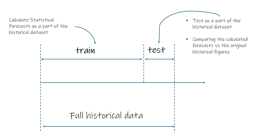
we calculate some statistical forecasts using the training part.
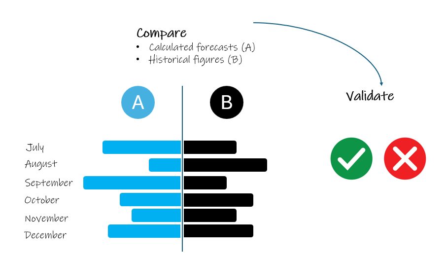
and we compare the calculated results for the last 6 months for example (see 2nd figure below).
- comparing the historical figures vs the calculated forecasts.
  - the closer the 2 figures are, the better.
- this approach also helps to identify the best statistical model.
  - comparing different algorithms.
  - or comparing different calculations for a same model, for example by choosing different training horizons.

43 Forecasts Performance

There are several ways to calculate the accuracy of forecasts, among them :

Mean Absolute Percentage Error (MAPE).
- Calculates the average of the absolute percentage errors between the forecast and the actual values.
- it is intuitive because it expresses accuracy as a percentage, making it easy to understand (e.g., a 5% MAPE means the average error is 5% of the actual value).
- A lower MAPE indicates a more accurate forecast.
- Formula: 𝑀𝐴𝑃𝐸=mean(|Actual−ForecastActual|)×100.
Mean Absolute Deviation (MAD).
- Calculates the average of the absolute differences between the forecast and actual values
- It provides the average error in the same units as the data (e.g., units of a product).
- It is best for comparing a single product’s accuracy, as using it for items with very different demand volumes can skew the results.
- A smaller MAD indicates a more accurate forecast.
- Formula: 𝑀𝐴𝐷=mean(|Actual−Forecast|).
Mean Square Error (MSE).
- Calculates the average of the squared errors between the forecast and actual values
- Squaring the errors penalizes larger errors more heavily than smaller ones.
- A smaller MSE indicates a better forecast.
- Formula: 𝑀𝑆𝐸=mean((Actual−Forecast)2).

We also need to consider the Forecasts Bias :

Measures the tendency of a forecast to consistently over or under estimate the actual value.
A negative bias indicates consistent under forecasting, while a positive bias indicates consistent over forecasting.
It is calculated by averaging the errors (actual minus forecast) without taking the absolute value.

Now, let’s practice and start calculating some statistical forecasts!