# ETL
library(tidyverse)

# for the tables
library(reactable)
library(reactablefmtr)

# for the charts
library(highcharter)

# Supply Chain
library(planr)

# Others
library(htmltools)28 DRP Calculation
First, let’s load a few libraries :
We’re going to present here how to use the drp() function from the R package planr.
This function allows to calculate a Replenishment Plan, also called DRP (Distribution Requirement Planning).
We need a dataset with the 5 classic variables to use this function :
a Product: it’s an item, a SKU (Storage Keeping Unit), or a SKU at a location, also called a DFU (Demand Forecast Unit).
a Period of time : for example monthly or weekly buckets.
a Demand : could be some sales forecasts, expressed in units.
an Opening Inventory : what we hold as available inventories at the beginning of the horizon, expressed in units.
a Supply Plan : the supplies that we plan to receive, expressed in units.
And a 4 new parameters added to this initial dataset :
SSCov: the Safety Stock Coverage, expressed in number of periods.DRPCovDur: the Frequency of Supply, expressed in number of periods.- it’s also the coverage duration that the replenishment plan represents.
MOQ: the Multiple Order Quantity, expressed in units, 1 by default or a multiple of a Minimum Order Quantity.FH: defines the Frozen and Free Horizon.It has 2 values: Frozen or Free.
If Frozen : no calculation of Replenishment Plan yet, the calculation starts when the period is defined as Free. We consider the existing supply plan in the Frozen Horizon.
We can use this parameter to consider some defined productions plans or supplies (allocations, workorders,…) in the short-term for example.
We are going to :
apply the function
drp()on a simple template.create 2 nice visuals of tables and charts to look at the results, using the R packages
reactable,reactablefmtrandhighcharter.
28.1 Demo data frame
First, let’s create a data frame which contains the basic features, i.e. the 5 variables :
2 dimensions : DFU & Period.
3 measures : Demand | Opening | Supply.
We’ll call it my_demand_and_suppply_data .
# create vectors
Period <- c(
"1/1/2020", "2/1/2020", "3/1/2020", "4/1/2020", "5/1/2020", "6/1/2020", "7/1/2020", "8/1/2020", "9/1/2020", "10/1/2020", "11/1/2020", "12/1/2020","1/1/2021", "2/1/2021", "3/1/2021", "4/1/2021", "5/1/2021", "6/1/2021", "7/1/2021", "8/1/2021", "9/1/2021", "10/1/2021", "11/1/2021", "12/1/2021")

Demand <- c(360, 458,300,264,140,233,229,208,260,336,295,226,336,434,276,240,116,209,205,183,235,312,270,201)

Opening <- c(1310,0,0,0,0,0,0,0,0,0,0,0,0,0,0,0,0,0,0,0,0,0,0,0)

Supply <- c(0,0,0,0,0,2500,0,0,0,0,0,0,0,0,0,2000,0,0,0,0,0,0,0,0)


# assemble
df1 <- data.frame(Period,
                  Demand,
                  Opening,
                  Supply)

# let's add a Product
df1$DFU <- "Product A"

# format the Period as a date
df1$Period <- as.Date(df1$Period, format = '%m/%d/%Y')

# keep results
my_demand_and_suppply_data <- df1

# let's have a look at it
head(my_demand_and_suppply_data)
Period Demand Opening Supply DFU
1 2020-01-01 360 1310 0 Product A
2 2020-02-01 458 0 0 Product A
3 2020-03-01 300 0 0 Product A
4 2020-04-01 264 0 0 Product A
5 2020-05-01 140 0 0 Product A
6 2020-06-01 233 0 2500 Product ANow, let’s add the 4 new parameters, that we will use to calculate the DRP :
SSCov: here 2 periods, means that we want to keep always, as a safety stocks, 2 months of coverage.DRPCovDur: here 3 periods, means that we want to replenish every 3 periods (it’s the frequency of replenishment).MOQ: here 1 unit, by default, so we keep a flexible Minimum Order Quantity.FH: here 6 first periods defined as Frozen, which means that the DRP calculation will start from the Period number 7, mentioned as Free.
We’ll call this final data frame my_drp_template_data .
# set a working df
df1 <- my_demand_and_suppply_data

# add DRP parameters
df1$SSCov <- 2
df1$DRPCovDur <- 3
df1$MOQ <- 1
df1$FH <- c("Frozen", "Frozen", "Frozen", "Frozen","Frozen","Frozen","Free","Free","Free","Free","Free","Free","Free","Free","Free","Free","Free","Free","Free","Free","Free","Free","Free","Free")


# get Results
my_drp_template_data <- df1

head(my_drp_template_data)
Period Demand Opening Supply DFU SSCov DRPCovDur MOQ FH
1 2020-01-01 360 1310 0 Product A 2 3 1 Frozen
2 2020-02-01 458 0 0 Product A 2 3 1 Frozen
3 2020-03-01 300 0 0 Product A 2 3 1 Frozen
4 2020-04-01 264 0 0 Product A 2 3 1 Frozen
5 2020-05-01 140 0 0 Product A 2 3 1 Frozen
6 2020-06-01 233 0 2500 Product A 2 3 1 Frozen28.2 DRP Calculation
Now let’s apply the function drp() to this data frame :
the initial input data frame my_drp_template_data, has 9 variables.
the output, called below calculated_drp, will have 15 variables.
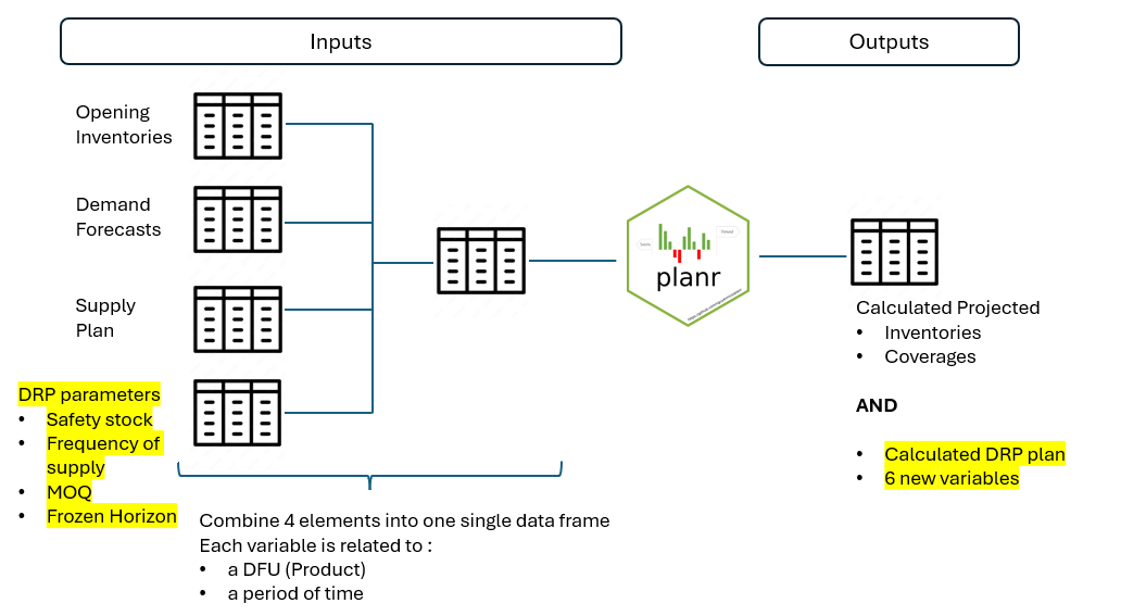
The 6 new variables are :
Stock.Max: sum of SSCov and DRPCovDur, expressed in periods of time.Safety.Stocks: the projected safety stocks, in units.Maximum.Stocks: the projected maximum stocks, in units.- Maximum Stock = Safety Stocks (SSCov) + Frequency of Supply (DRPCovDur)
DRP.Calculated.Coverage.in.Periods: the calculated projected inventories, expressed in periods of time.DRP.Projected.Inventories.Qty: the calculated projected inventories, based on theDRP.plan.DRP.plan: the calculated Replenishment Plan.- in the Frozen Horizon : equal to the existing plan, which is “frozen”.
- in the Free Horizon : the calculated plan, based on the parameters
SSCov|DRPCovDur|MOQ.
# set a working df
df1 <- my_drp_template_data

# calculate drp
df1 <- planr::drp(data = df1,
                  DFU = DFU,
                  Period = Period,

                  Demand =  Demand,
                  Opening = Opening,
                  Supply = Supply,

                  SSCov = SSCov,
                  DRPCovDur = DRPCovDur,
                  MOQ = MOQ,
                  FH = FH)

# keep results
calculated_drp <- df1

glimpse(calculated_drp)
Rows: 24
Columns: 15
$ DFU <chr> "Product A", "Product A", "Product …
$ Period <date> 2020-01-01, 2020-02-01, 2020-03-01…
$ Demand <dbl> 360, 458, 300, 264, 140, 233, 229, …
$ Opening <dbl> 1310, 0, 0, 0, 0, 0, 0, 0, 0, 0, 0,…
$ Supply <dbl> 0, 0, 0, 0, 0, 2500, 0, 0, 0, 0, 0,…
$ SSCov <dbl> 2, 2, 2, 2, 2, 2, 2, 2, 2, 2, 2, 2,…
$ DRPCovDur <dbl> 3, 3, 3, 3, 3, 3, 3, 3, 3, 3, 3, 3,…
$ Stock.Max <dbl> 5, 5, 5, 5, 5, 5, 5, 5, 5, 5, 5, 5,…
$ MOQ <dbl> 1, 1, 1, 1, 1, 1, 1, 1, 1, 1, 1, 1,…
$ FH <chr> "Frozen", "Frozen", "Frozen", "Froz…
$ Safety.Stocks <dbl> 758, 564, 404, 373, 462, 437, 468, …
$ Maximum.Stocks <dbl> 1395, 1166, 1074, 1070, 1266, 1328,…
$ DRP.Calculated.Coverage.in.Periods <dbl> 2.7, 1.7, 0.7, 0.0, 0.0, 7.4, 6.4, …
$ DRP.Projected.Inventories.Qty <dbl> 950, 492, 192, -72, -212, 2055, 182…
$ DRP.plan <dbl> 0, 0, 0, 0, 0, 2500, 0, 0, 0, 0, 0,…The inputs | outputs are displayed in the picture below :
28.3 DRP Table
First, let’s create a function status_PI.Index() .
# create a function status.PI.Index
status_PI.Index <- function(color = "#aaa", width = "0.55rem", height = width) {
  span(style = list(
    display = "inline-block",
    marginRight = "0.5rem",
    width = width,
    height = height,
    backgroundColor = color,
    borderRadius = "50%"
  ))
}
Now let’s create a table, using the packages reactable and reactablefmtr .
This table is pretty similar to the ones we saw previously, while describing the functions light_proj_inv() and proj_inv() .
The main differences are :
a variable related to the Frozen Horizon.
the output of the calculated DRP plan.
# set a working df
df1 <- calculated_drp

# keep only the needed columns
df1 <- df1 |> select(Period,
                     FH,
                     Demand,
                     DRP.Calculated.Coverage.in.Periods,
                     DRP.Projected.Inventories.Qty,
                     DRP.plan)


# replace missing values by zero
df1$DRP.plan <- df1$DRP.plan |> replace_na(0)
df1$DRP.Projected.Inventories.Qty <- df1$DRP.Projected.Inventories.Qty |> replace_na(0)

# create a f_colorpal field
df1 <- df1 |> mutate(f_colorpal = case_when(
  DRP.Calculated.Coverage.in.Periods > 8 ~ "#FFA500",
  DRP.Calculated.Coverage.in.Periods > 2 ~ "#32CD32",
  DRP.Calculated.Coverage.in.Periods > 0 ~ "#FFFF99",
  TRUE ~ "#FF0000" )
  )


# create reactable
reactable(df1, resizable = TRUE, showPageSizeOptions = TRUE,

              striped = TRUE, highlight = TRUE, compact = TRUE,
              defaultPageSize = 20,

              columns = list(


                FH = colDef(
                  name = "Frozen Horizon",

                  cell = function(value) {
                    color <- switch(
                      value,
                      Free = "hsl(154, 64%, 50%)",
                      Frozen = "hsl(3, 69%, 50%)"
                    )
                    PI.Index <- status_PI.Index(color = color)
                    tagList(PI.Index, value)
                  }),

                Demand = colDef(
                  name = "Demand (units)",

                  cell = data_bars(df1,
                                   fill_color = "#3fc1c9",
                                   text_position = "outside-end"
                  )

                ),

              DRP.Calculated.Coverage.in.Periods = colDef(
                name = "Coverage (Periods)",
                maxWidth = 90,
                cell= color_tiles(df1, color_ref = "f_colorpal")
              ),

              f_colorpal = colDef(show = FALSE), # hidden, just used for the coverages

                `DRP.Projected.Inventories.Qty`= colDef(
                  name = "Projected Inventories (units)",
                  format = colFormat(separators = TRUE, digits=0),

                  style = function(value) {
                    if (value > 0) {
                      color <- "#008000"
                    } else if (value < 0) {
                      color <- "#e00000"
                    } else {
                      color <- "#777"
                    }
                    list(color = color
                         #fontWeight = "bold"
                    )
                  }
                ),

              DRP.plan = colDef(
                name = "Replenishment (units)",
                cell = data_bars(df1,
                                 fill_color = "#3CB371",
                                 text_position = "outside-end"
                                 )
                )

              ), # close columns list

              columnGroups = list(

                colGroup(name = "Projected Inventories",
                         columns = c("DRP.Calculated.Coverage.in.Periods",
                                     "DRP.Projected.Inventories.Qty")
                         )

              )

    ) # close reactable
28.4 DRP charts
We can also visualize the result through a chart, using the library highcharter.
28.4.1 Line Chart
# set a working df
df1 <- calculated_drp

# Chart
highchart() |>

  hc_add_series(name = "Max",
                color = "crimson",
                data = df1$Maximum.Stocks) |>

  hc_add_series(name = "min",
                color = "lightblue",
                data = df1$Safety.Stocks) |>

  hc_add_series(name = "Projected Inventories",
                color = "gold",
                data = df1$DRP.Projected.Inventories.Qty) |>

  hc_title(text = "(DRP) Projected Inventories") |>
  hc_subtitle(text = "in units") |>

  hc_xAxis(categories = df1$Period) |>
  hc_add_theme(hc_theme_google())
We can notice that the Frozen Horizon is until “2020-06-01” included. Until this period, we consider the current supply plan.
Within this Frozen Horizon we have an Out of Stocks period during “2020-04-01” and “2020-05-01”, following by an overstock situation in “2020-06-01” and “2020-07-01”.
Then the DRP calculation generates a replenishment plan which is always the 2 min and max stocks targets in the coming months.
28.4.2 Bar Chart
We can display the same type of chart we created before, with Positive & Negative Projected Inventories.
This puts more focus on the eventual shortages.
# set a working df
df1 <- calculated_drp

# keep only the needed columns
df1 <- df1 |> select(Period, DRP.Projected.Inventories.Qty)

# create a value.index
df1$Value.Index <- if_else(df1$DRP.Projected.Inventories.Qty < 0, "Shortage", "Stock")


# spread
df1 <- df1 |> spread(Value.Index, DRP.Projected.Inventories.Qty)


#------------------
# Chart
#------------------

highchart() |>
  hc_title(text = "Projected Inventories") |>
  hc_subtitle(text = "in units") |>
  hc_add_theme(hc_theme_google()) |>

  hc_xAxis(categories = df1$Period) |>

  hc_add_series(name = "Stock",
                color = "#32CD32",
                #dataLabels = list(align = "center", enabled = TRUE),
                data = df1$Stock) |>

  hc_add_series(name = "Shortage",
                color = "#dc3220",
                #dataLabels = list(align = "center", enabled = TRUE),
                data = df1$Shortage) |>

  hc_chart(type = "column") |>
  hc_plotOptions(series = list(stacking = "normal"))