c("a", "b", "c", "d")[1] "a" "b" "c" "d"first things first : Upload libraries
It’s a good practice to start a quarto document (or a R file) by loading the libraries we will use. Those libraries can be related to the ETL, the Data Visualization (Charts, Tables), some special calculations, shiny web apps, etc…
Here, we will start practicing on the ETL, and will load very often the R package tidyverse.
The tidyverse is a collection of inter-operable R packages for data science that share a common design philosophy, grammar, and data structures. This package is one of the reasons why R is so popular for data manipulation capabilities.
Among those packages, we have :
dplyr : Data manipulation (wrangling).
tidyr : Data tidying of CSV or TSV files.
stringr : String manipulation, provides a cohesive set of functions for working with character data.
forcats : Factor manipulation.
lubridate : simplifies working with dates and times.
To load the tidyverse library, we write the syntax library(tidyverse) :
Everything is an object: In R, virtually everything, including functions, vectors, and lists, is an object. An object’s class defines its structure.
In this part, we are going to look at the main objects that we will use in R :
vectors.
data frames.
And the different classes of variables which composed those objects, with a particular focus on :
factor.
list.
We will learn :
how to create data frames, and to upload data (from a csv or an excel file) and write them (into a csv or an excel file)
the very basic syntax to :
create an object.
access a particular variable of a data frame.
We will also introduce some first functions, such as :
data.frame() : to create a data frame.
as.Date() : to create a date.
class() : to check the class of an object.
str() : to check the content (the structure) of an object.
A function is a word, which performs an operation. It is displayed as the name of the function followed by 2 parentheses (). The function is applied to an object, or some variables of it, which are placed between the 2 parentheses.
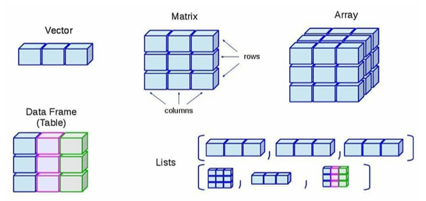
different data structures
R handles several types of Data Structures, especially :
vector.
data frame.
matrix.
array.
list.
Through this book, we will use mainly vectors, data frames, and lists.
different classes
A class characterizes the format of the values which are contained inside a data structure, or the data structure itself.
Most common ones are:
numeric.
integer.
character.
factor.
date.
logical.
list.
And of course :
We will look at them gradually more in details in the coming parts.
It’s the most basic object, and a key element, in the R ecosystem.
It’s also the component of other objects, such as data frames or lists.
To create a vector, we just need to type the syntax below :
start with the letter “c” and add 2 parentheses : c() .
then between parentheses, write some elements, separated by a comma .
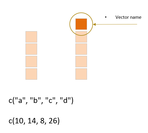
Let’s create our first vector, composed of characters :
c("a", "b", "c", "d")[1] "a" "b" "c" "d"Note : if we want to handle some characters, we need to put them between 2 quotes ““ .
For example :
100 will be captured as a numeric value.
whereas “100” will be captured as a character.
Here is a vector with numeric values :
c(10, 14, 8, 26)[1] 10 14 8 26We have created 2 vectors, but we can’t see them as existing objects : they don’t appear in our environment, in the top right panel of our IDE.
In order to use them later on, we need to affect an object, through a name, to those vectors.
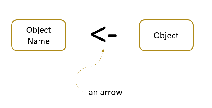
To affect an object name to a vector, we simply use the syntax below :
First we define a name for our object, and then using an arrow, written “<-” we affect an object, here a vector, to it.
This object can also be a data frame or a list, as we will see later on.
Let’s practice :
We create an object call “people”.
# create vector
people <- c("Seb", "Max", "Nico", "Greg")
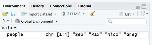
Note that this object now appears on the top right of your IDE, in your environment. It means that it exists (in your environment) : you can access it and you can use it later on.
We get an overview of it, and can notice some useful information :
its class is a character : it’s written “chr” at the beginning.
it contains 1 to 4 elements : it’s written between bracket [1:4].
a snapshot of the first elements is displayed : “Seb” “Max” “Nico” “Greg”.
You also can type in a chunk of a quarto document the name of the object, and it will be displayed below the chunk :
# display
people
[1] "Seb" "Max" "Nico" "Greg"Let’s look at the class of this vector :
class(people)[1] "character"Let’s have another example, this time using some numerical values :
# create vector
age <- c(10, 14, 8, 26)

# display
age
[1] 10 14 8 26A data frame is like a table, composed of vectors.
the vectors are the columns, that we will call more specifically variables.
the vectors’ names are the variables’ names.
It’s what we (very) often use in excel.
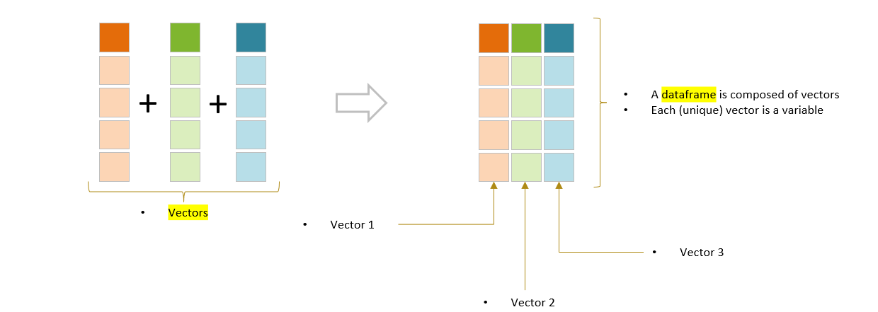
So we can create a data frame by combining some vectors.
Here is one way, creating the vectors first and them combining them into a data frame :
we create first 2 vectors of 4 elements each.
we assemble them into a data frame with the function data.frame().
# create vectors
people <- c("Tom", "Max", "Nico", "Greg")
age <- c(10, 14, 8, 26)

# combine them into a dataframe, using the data.frame() function
mydataframe <- data.frame(
  people,
  age
  )

# display
mydataframe
people age
1 Tom 10
2 Max 14
3 Nico 8
4 Greg 26We can use the function glimpse() to display an overview of the data frame and also get some information about the class of each variable, next to its name :
glimpse(mydataframe)Rows: 4
Columns: 2
$ people <chr> "Tom", "Max", "Nico", "Greg"
$ age <dbl> 10, 14, 8, 26next to people : “chr” stands for “character”.
next to age : “dbl” stands for “double”, i.e. a numerical value.
Here is another way to create a data frame, creating the variables straight into a data.frame() function :
# create straight away the dataframe
mydataframe <- data.frame(
people = c("Tom", "Max", "Nico", "Greg"),
age = c(10, 14, 8, 26)
)
# display
mydataframe people age
1 Tom 10
2 Max 14
3 Nico 8
4 Greg 26Let’s look at the class of the object “mydataframe” : it’s a data.frame
class(mydataframe)[1] "data.frame"Let’s explore a bit the RStudio IDE.
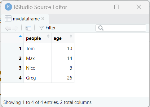
We can click on the name of object on the top right of the RStudio IDE, in the Environment tab, and the object will appear in a new window.
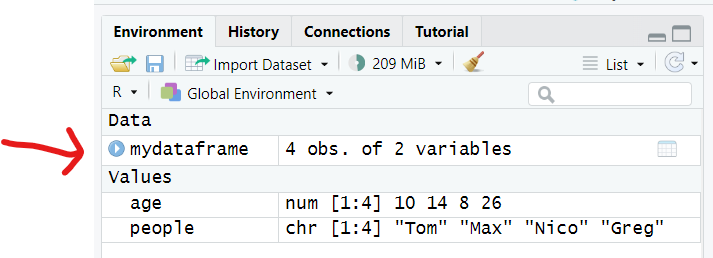
It now appears in a new tab or window in the top left panel of RStudio. You can click on it to display it.
You can :
click on the variables’ names to sort the data.
click on the Filter button to display some “search” boxes below the variables’ names and filter some data.
We also have a few info about the data frame on its bottom left :
number of entries (i.e. the rows) which are displayed.
number of columns of the data frame.
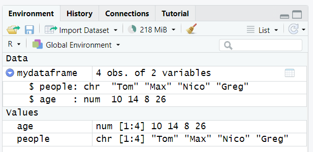
In the Environment tab, you can click on the little blue arrow on the left (of the object) to see the composition of the data frame :
first variable is a vector of characters.
second variable is a vector of numerical values.
We now have a data frame, and we will be able to perform some manipulations and calculations on it later on.
We can select a variable of a data frame using the syntax object_name$variable_name .
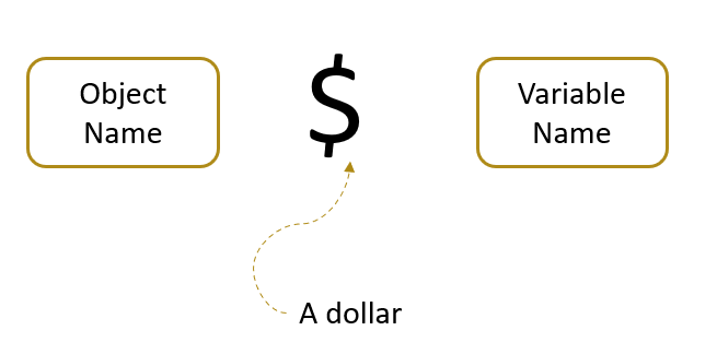
Using our previous data frame, let’s select the variable “people” :
# select the variable "people"
mydataframe$people[1] "Tom" "Max" "Nico" "Greg"It might be at the beginning a bit challenging to figure out what is a list.
We often describe a list as a train.
A list is group of different elements, and those elements can be of different types (i.e class). Each element has a location within the list, like inside the cars of a train.
For example, we can have inside a list :
a vector.
but also a vector and a data frame.
or several lists.
…
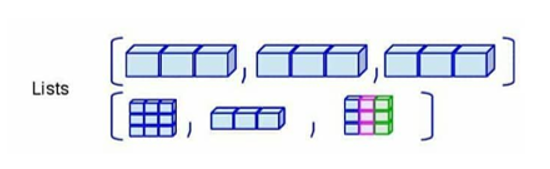
To illustrate it, let’s create a list composed of 2 elements :
the vector called “people”.
the data.frame called “mydataframe”.
We will use the function list() to generate this object.
# create list
mylist <- list(people, mydataframe)
# display list
mylist[[1]]
[1] "Tom" "Max" "Nico" "Greg"
[[2]]
  people age
1    Tom  10
2    Max  14
3   Nico   8
4   Greg  26
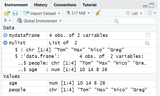
We can see that the object “mylist” appears here with 2 elements. Each element is located at a specific position.
To access one element located inside a specific position, we simply need to write : the name of the object (i.e. the list) and between 2 square brackets the location.
For example, to get the data frame which is located in the second position, we will write :
mylist[[2]] people age
1 Tom 10
2 Max 14
3 Nico 8
4 Greg 26or to get the vector:
mylist[[1]][1] "Tom" "Max" "Nico" "Greg"The object “mylist” now appears on the top right of the RStudio IDE.
You can click on the little arrow on the left to see its composition :
first location contains a vector of characters.
second location contains a data frame.
The list class is a very flexible class, and is very useful to perform some analysis or to create some particular displays in some tables, such as sparklines. We will practice in the next chapters.
As we saw before in the section data structures, we can put anything inside a list, such as numbers:
list1 <- list(3, 2)

list1
[[1]]
[1] 3
[[2]]
[1] 2Or other vectors constructed with c():
list2 <- list(c(1, 2), c(3, 4))

list2
[[1]]
[1] 1 2
[[2]]
[1] 3 4You can also put objects of different classes in the same list:
list3 <- list(3, c(1, 2), "lists are amazing!")

list3
[[1]]
[1] 3
[[2]]
[1] 1 2
[[3]]
[1] "lists are amazing!"And of course create list of lists:
my_lists <- list(list1, list2, list3)

my_lists
[[1]]
[[1]][[1]]
[1] 3
[[1]][[2]]
[1] 2
[[2]]
[[2]][[1]]
[1] 1 2
[[2]][[2]]
[1] 3 4
[[3]]
[[3]][[1]]
[1] 3
[[3]][[2]]
[1] 1 2
[[3]][[3]]
[1] "lists are amazing!"To check the contents of a list, you can use the structure function str() :
str(my_lists)List of 3
$ :List of 2
..$ : num 3
..$ : num 2
$ :List of 2
..$ : num [1:2] 1 2
..$ : num [1:2] 3 4
$ :List of 3
..$ : num 3
..$ : num [1:2] 1 2
..$ : chr "lists are amazing!"And you can use the function class() to check the class of the object :
class(my_lists)[1] "list"We already saw a few types of classes so far : characters, numerical values, data frames and lists.
Numerical values can be :
integer.
double (i.e a numerical values which is not an integer).
There are also 3 very useful classes :
date.
factor.
logical.
Remember that to check the class of an object, we can use the function class().
We will see through this book that R allows us to handle very easily dates coming in very different formats, especially using the package lubridate.
For the time being, let’s notice how is identified the class of a date object.
First, let’s create a date, as a character :
# create date, in the format MM/DD/YYY
mydate <- "05/01/2025"

# display
mydate
[1] "05/01/2025"Now, let’s convert it into a proper date, using the function as.Date():
# convert as a date
mydate <- as.Date(mydate, format = '%m/%d/%Y')

# display
mydate
[1] "2025-05-01"The display is already different from previously, and “mydate” now appears in a standardized format : YYYY-MM-DD
We can check the class :
class(mydate)[1] "Date"Week of the year
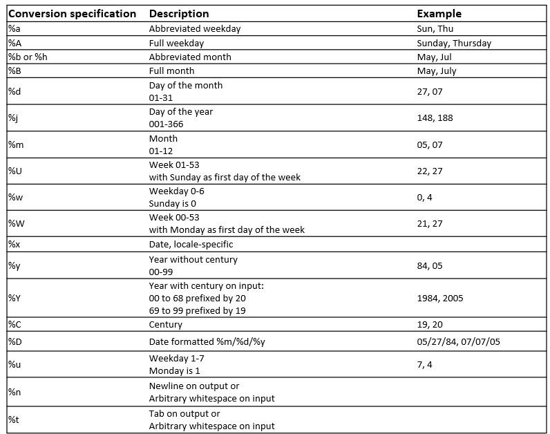
US convention: Week of the year as decimal number (00-53) using Sunday as the first day 1 of the week (and typically with the first Sunday of the year as day 1 of week 1): %U
UK convention: Week of the year as decimal number (00-53) using Monday as the first day of week (and typically with the first Monday of the year as day 1 of week 1): %W
ISO 8601 definition: Week of the year as decimal number (01-53) as defined in ISO 8601.
If the week (starting on Monday) containing 1 January has four or more days in the new year, then it is considered week 1.
Otherwise, it is the last week of the previous year, and the next week is week 1: % which is accepted but ignored on input.
Note that there is also a week-based year (%G and %g ) which is to be used with %V as it may differ from the calendar year (%Y and %y ).
Numeric weekday
Weekday as a decimal number (1-7, Monday is 1): %u
Weekday as decimal number (0-6, Sunday is 0): %w
Interestingly, there is no format for the case Sunday is counted as day 1 of the week.
In the table below are the main dates conversions that we will use through this book.
Here comes a super useful type of class.
To illustrate it, imagine that we are working for a company who is using a Fiscal Calendar, with the month of October as first month of this fiscal year.
We can create an object (data frame), called fiscal_calendar_data as below :
# create calendar
fiscal_calendar_data <- data.frame(

  calendar_month_abb = c("Oct", "Nov", "Dec", "Jan", "Feb", "Mar",
                         "Apr", "May", "Jun", "Jul", "Aug", "Sep"),

  fiscal_month = c(1,2,3,4,5,6,7,8,9,10,11,12)
  )

# display
fiscal_calendar_data
calendar_month_abb fiscal_month
1 Oct 1
2 Nov 2
3 Dec 3
4 Jan 4
5 Feb 5
6 Mar 6
7 Apr 7
8 May 8
9 Jun 9
10 Jul 10
11 Aug 11
12 Sep 12We notice that the variable “calendar_month_abb” is a character.
Let’s open it, by clicking on the object fiscal_calendar_data in our Environment (top right). Now, we can click on the variable calendar_month_abb : it allows us to sort the different elements.
We notice that the different elements are sorted according to an alphabetical order (from start to end or the opposite). It’s because the class is a character.
We can change this, by modifying the class of the variable calendar_month_abb, into a factor.
We will define levels, to indicate a new order for this variable
# create a Factor for the variable calendar_month_abb
# setting the beginning to October, to reflect the beginning of a Fiscal Year
fiscal_calendar_data$calendar_month_abb <- factor(
  fiscal_calendar_data$calendar_month_abb,

    levels = c("Oct", "Nov", "Dec", "Jan","Feb","Mar",
               "Apr","May","Jun","Jul","Aug","Sep")
  )
Now let’s look again at our object fiscal_calendar_data :
# display
fiscal_calendar_data
calendar_month_abb fiscal_month
1 Oct 1
2 Nov 2
3 Dec 3
4 Jan 4
5 Feb 5
6 Mar 6
7 Apr 7
8 May 8
9 Jun 9
10 Jul 10
11 Aug 11
12 Sep 12The variable calendar_month_abb has a class “fctr” which stands for factor.
When we sort it, it starts from October, and ends in September.
A factor is a bit like having an attribute (here called a level), on top of a value (here a month, in character).
This will be for example pretty convenient to display some charts (continuing the example of this dataset).
This class is the result of logical comparisons, for example, if you type:
# create a test
4 > 3
[1] TRUER returns TRUE, which is an object of class logical:
# affect an object called "k" to this test
k <- 4 > 3

# check the class of the object k
class(k)
[1] "logical"In other programming languages, logicals are often called bools.
A logical variable can only have two values, either TRUE or FALSE.
You can test the truthfulness of a variable with the function isTRUE() :
k <- 4 > 3
isTRUE(k)
[1] TRUEHow can you test if a variable is false?
There is not a isFALSE() function (at least not without having to load a package containing this function), but there is way to do it, adding a “!” before the the function isTRUE():
k <- 4 > 3
!isTRUE(k)
[1] FALSEThe ! operator indicates negation, so the above expression could be translated as is k not TRUE?