# ETL
library(tidyverse)
library(sparkline)

# Tables
library(reactable)
library(reactablefmtr)

# Charts
library(highcharter)

# Supply Chain
library(planr)33 Projected In Transit
Let’s upload the libraries we’re going to use :
Objectives
To show how to use the proj_git()function from the planr package.
Note : “proj_git” stands for “Projection Goods In Transit”.
The idea is to calculate, considering a Transit Time, the projected inventories in transit.
34 Demo dataset
Overview
Let’s use the built-in demo dataset demo_in_transit from the planr package.
It contains 6 variables :
DFU: a location and an item.- there are 3 DFUs : Entity 1_Product A / Entity 2_Product B / Entity 3_Product C.
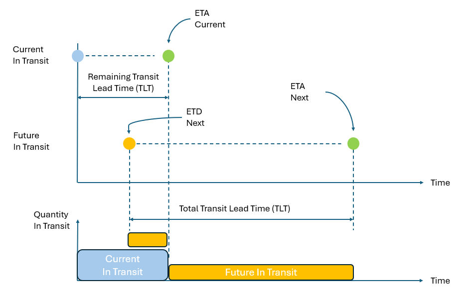
Period: a date in weekly bucket format.ETA.CurrentETA stands for Estimated Time of Arrival.
some quantities currently in transit displayed at their ETA date in units.
ETA.Next- some quantities to be shipped, not yet in transit, displayed at their ETA date in units.
ETD.NextETD stands for Estimated Time of Departure.
some quantities to be shipped, not yet in transit, displayed at their ETD date in units.
TLTthe Transit Lead Time, expressed in weeks.
represents the difference between ETA and ETD dates.
There are 2 types of in transit :
the current in transit.
the next one, not yet shipped.
Note that the difference between ETD and ETA is the Transit Time.
In this tutorial, we will use this data frame to project the Goods In Transit.
We will apply on this data frame the proj_git() function. It will calculate the variable Proj.GIT which gathers the current and next In Transit quantities.
The concept is illustrated in the figure below.
The total projected quantity in transit is the sum of the [current in transit] and the [future in transit].
data("demo_in_transit")

head(demo_in_transit)
# A tibble: 6 × 6
DFU Period ETA.Current ETA.Next ETD.Next TLT
<chr> <date> <dbl> <dbl> <dbl> <dbl>
1 Entity 1_Product A 2024-02-18 0 0 0 8
2 Entity 1_Product A 2024-02-25 1008 0 500 8
3 Entity 1_Product A 2024-03-03 0 0 0 8
4 Entity 1_Product A 2024-03-10 252 0 0 8
5 Entity 1_Product A 2024-03-17 0 0 0 8
6 Entity 1_Product A 2024-03-24 0 0 800 8Summary DFUs x Transit Time
Let’s display the Transit Lead Times (TLT) for each DFU, expressed in number of weeks.
We have 3 different couples Entity x Product, with 3 different Transit Times :
a long one : 8 weeks, for Entity 1_Product A.
a medium one : 4 weeks, for Entity 2_Product B.
a short one : 2 weeks, Entity 3_Product C.
# keep only unique variables
df1 <- demo_in_transit |> group_by(DFU) |>
  summarise(TLT = mean(TLT)
            )
# display
df1
# A tibble: 3 × 2
DFU TLT
<chr> <dbl>
1 Entity 1_Product A 8
2 Entity 2_Product B 4
3 Entity 3_Product C 235 Calculate Projected In Transit
Using the proj_git() function, we can calculate the Projected In Transit for all the different couples Entity x Product contained into the data frame.
# apply proj_git()
df1 <- planr::proj_git(
  dataset = demo_in_transit,
  DFU = DFU,
  Period = Period,
  ETA.Current = ETA.Current,
  ETA.Next = ETA.Next,
  ETD.Next = ETD.Next,
  TLT = TLT)

# keep results
calculated_GIT_data <- df1

glimpse(calculated_GIT_data)
Rows: 447
Columns: 11
$ DFU <chr> "Entity 1_Product A", "Entity 1_Product A", "Entity 1…
$ Period <date> 2024-02-18, 2024-02-25, 2024-03-03, 2024-03-10, 2024…
$ ETA.Current <dbl> 0, 1008, 0, 252, 0, 0, 0, 0, 0, 0, 0, 0, 0, 0, 0, 0, …
$ ETA.Next <dbl> 0, 0, 0, 0, 0, 0, 0, 0, 0, 500, 0, 0, 0, 800, 0, 0, 0…
$ ETD.Next <dbl> 0, 500, 0, 0, 0, 800, 0, 0, 0, 600, 0, 0, 0, 0, 0, 0,…
$ TLT <dbl> 8, 8, 8, 8, 8, 8, 8, 8, 8, 8, 8, 8, 8, 8, 8, 8, 8, 8,…
$ Current.GIT <dbl> 1260, 0, 0, 0, 0, 0, 0, 0, 0, 0, 0, 0, 0, 0, 0, 0, 0,…
$ ETD.Current <dbl> 0, 0, 0, 0, 0, 0, 0, 0, 0, 0, 0, 0, 0, 0, 0, 0, 0, 0,…
$ Proj.Current.GIT <dbl> 1260, 252, 252, 0, 0, 0, 0, 0, 0, 0, 0, 0, 0, 0, 0, 0…
$ Proj.Future.GIT <dbl> 0, 500, 500, 500, 500, 1300, 1300, 1300, 1300, 1400, …
$ Proj.GIT <dbl> 1260, 752, 752, 500, 500, 1300, 1300, 1300, 1300, 140…We get 5 new variables:
Current.GIT: the total inventories currently in transit.ETD.Current: estimated Departure Time when the current inventories in transit were shipped.Proj.Current.GIT: projected inventories of the current in transit.Proj.Future.GIT: projected inventories of the future in transit.Proj.GIT: total projected inventories, current and future in transit.
Those variables will be useful to display the projection of the inventories in transit.
36 Visualize
36.1 Individual Projections
For our 3 different DFUs, let’s visualize the projection of the In Transit inventories.
There are 2 components to consider :
Current in transit.
Future in transit.
We observe (as expected!) that the longer the transit time, the higher the projected in transit.
36.1.1 Entity 1 x Product A
# set a working df
df1 <- calculated_GIT_data

# filter
df1 <- filter(df1, df1$DFU == "Entity 1_Product A")

# make the horizon shorter
df1 <- filter(df1, df1$Period <= (min(df1$Period) + 120) )

#--------------------
# Chart

highchart() |>

  hc_title(text = "Projected In Transit") |>
  hc_subtitle(text = "in units") |>
  hc_add_theme(hc_theme_google()) |>

  hc_xAxis(categories = df1$Period) |>

  hc_add_series(name = "Current",
                color = "steelblue",
                dataLabels = list(align = "center", enabled = TRUE),
                data = df1$Proj.Current.GIT) |>


  hc_add_series(name = "Future",
                color = "gold",
                dataLabels = list(align = "center", enabled = TRUE),
                data = df1$Proj.Future.GIT) |>

  hc_chart(type = "column") |>
  hc_plotOptions(series = list(stacking = "normal"))
36.1.2 Entity 2 x Product B
# set a working df
df1 <- calculated_GIT_data

# filter
df1 <- filter(df1, df1$DFU == "Entity 2_Product B")

# make the horizon shorter
df1 <- filter(df1, df1$Period <= (min(df1$Period) + 120) )

#--------------------
# Chart

highchart() |>

  hc_title(text = "Projected In Transit") |>
  hc_subtitle(text = "in units") |>
  hc_add_theme(hc_theme_google()) |>

  hc_xAxis(categories = df1$Period) |>

  hc_add_series(name = "Current",
                color = "steelblue",
                dataLabels = list(align = "center", enabled = TRUE),
                data = df1$Proj.Current.GIT) |>


  hc_add_series(name = "Future",
                color = "gold",
                dataLabels = list(align = "center", enabled = TRUE),
                data = df1$Proj.Future.GIT) |>

  hc_chart(type = "column") |>
  hc_plotOptions(series = list(stacking = "normal"))
36.1.3 Entity 3 x Product C
# set a working df
df1 <- calculated_GIT_data

# filter
df1 <- filter(df1, df1$DFU == "Entity 3_Product C")

# make the horizon shorter
df1 <- filter(df1, df1$Period <= (min(df1$Period) + 120) )

#--------------------
# Chart

highchart() |>

  hc_title(text = "Projected In Transit") |>
  hc_subtitle(text = "in units") |>
  hc_add_theme(hc_theme_google()) |>

  hc_xAxis(categories = df1$Period) |>

  hc_add_series(name = "Current",
                color = "steelblue",
                dataLabels = list(align = "center", enabled = TRUE),
                data = df1$Proj.Current.GIT) |>


  hc_add_series(name = "Future",
                color = "gold",
                dataLabels = list(align = "center", enabled = TRUE),
                data = df1$Proj.Future.GIT) |>

  hc_chart(type = "column") |>
  hc_plotOptions(series = list(stacking = "normal"))
36.2 Comparison
Let’s compare on a same chart the different quantities in transit.
As mentioned previously the longer the Transit Lead Time, the bigger are the projected inventories in transit.
a 8 weeks lead time means here almost every week some stocks in transit.
while a 2 weeks lead time shows some periods of time without any volume in transit.
This calculation makes also easy the projection of the Total Inventories of a supply network.
For example if Entity 1 supplies a Product A to the Entity 2, we could :
project the local inventories at the Entity 1.
project the local inventories at the Entity 2.
and also project the inventories in transit between both entities.
# set a working df
df1 <- calculated_GIT_data

# filter : make the horizon shorter
df1 <- filter(df1, df1$Period <= (min(df1$Period) + 120) )

# keep only needed variables
df1 <- df1 |> select(DFU, Period, Proj.GIT)

# spread
df1 <- df1 |> spread(DFU, Proj.GIT)


#--------------------
# Chart

highchart() |>

  hc_add_series(name = "8 weeks",
                color = "gold",
                dataLabels = list(align = "center", enabled = TRUE),
                data = df1$`Entity 1_Product A`) |>

  hc_add_series(name = "4 weeks",
                color = "steelblue",
                dataLabels = list(align = "center", enabled = TRUE),
                data = df1$`Entity 2_Product B`) |>

  hc_add_series(name = "2 weeks",
                color = "mediumseagreen",
                dataLabels = list(align = "center", enabled = TRUE),
                data = df1$`Entity 3_Product C`) |>

  hc_title(text = "Comparison Projected In Transit") |>
  hc_subtitle(text = "in units") |>

  hc_xAxis(categories = df1$Calendar.Month.abb) |>

  hc_add_theme(hc_theme_google())
36.3 All In Transit
If we want to calculate the total quantities in transit for our 3 couples Entity x Product, we can simply sum them.
The chart below illustrates this idea.
Interesting to visualize where are the most important projected inventories in transit for a supply network :
which products.
between which entities.
how much inventories.
# set a working df
df1 <- calculated_GIT_data

# filter : make the horizon shorter
df1 <- filter(df1, df1$Period <= (min(df1$Period) + 120) )

# keep only needed variables
df1 <- df1 |> select(DFU, Period, Proj.GIT)

# spread
df1 <- df1 |> spread(DFU, Proj.GIT)


#--------------------
# Chart

highchart() |>

  hc_title(text = "Projected All In Transit") |>
  hc_subtitle(text = "in units") |>
  hc_add_theme(hc_theme_google()) |>

  hc_xAxis(categories = df1$Period) |>


  hc_add_series(name = "8 weeks",
                color = "gold",
                dataLabels = list(align = "center", enabled = TRUE),
                data = df1$`Entity 1_Product A`) |>


  hc_add_series(name = "4 weeks",
                color = "steelblue",
                dataLabels = list(align = "center", enabled = TRUE),
                data = df1$`Entity 2_Product B`) |>

  hc_add_series(name = "2 weeks",
                color = "mediumseagreen",
                dataLabels = list(align = "center", enabled = TRUE),
                data = df1$`Entity 3_Product C`) |>

  hc_chart(type = "column") |>
  hc_plotOptions(series = list(stacking = "normal"))
37 DRP and In Transit
Let’s now project the inventories in transit in the context of a DRP.
We can consider the Entity 1 x Product A.
The idea is to then visualize together 2 parts :
local projected inventories.
projected in-transit.
- which often, once shipped, belongs financially to the receiving Entity 1.
It’s an easy way to simulate, based on some DRP parameters (and also the Demand Forecasts) the total (local + in transit) projected inventories of an Entity.
Let’s prepare our data frame to calculate our DRP. We need to add :
- 3 variables related to the Demand | Opening | Supply.
- the DRP parameters : SSCov | DRPCovDur | MOQ | FH (Frozen Horizon).
#--------------------
# Add Demand / Opening / Supply
#--------------------


# set a working df
df1 <- calculated_GIT_data

# filter
df1 <- filter(df1, df1$DFU == "Entity 1_Product A")

# add Demand
df1$Demand <- 100

# add Supply
df1$Supply <- 0

# add Opening
df1$Opening <- if_else(df1$Period == min(df1$Period), 600, 0)
df1$Opening <- df1$Opening |> replace_na(0)

# keep only needed variables
df1 <- df1 |> select(DFU,
                     Period,
                     Demand,
                     Opening,
                     Supply)


#--------------------
# Add DRP parameters
#--------------------

df1$SSCov <- 2
df1$DRPCovDur <- 3

df1$MOQ <- 1
df1$FH <- if_else(df1$Period <= '2024-04-07', "Frozen", "Free")


glimpse(df1)
Rows: 149
Columns: 9
$ DFU <chr> "Entity 1_Product A", "Entity 1_Product A", "Entity 1_Produc…
$ Period <date> 2024-02-18, 2024-02-25, 2024-03-03, 2024-03-10, 2024-03-17,…
$ Demand <dbl> 100, 100, 100, 100, 100, 100, 100, 100, 100, 100, 100, 100, …
$ Opening <dbl> 600, 0, 0, 0, 0, 0, 0, 0, 0, 0, 0, 0, 0, 0, 0, 0, 0, 0, 0, 0…
$ Supply <dbl> 0, 0, 0, 0, 0, 0, 0, 0, 0, 0, 0, 0, 0, 0, 0, 0, 0, 0, 0, 0, …
$ SSCov <dbl> 2, 2, 2, 2, 2, 2, 2, 2, 2, 2, 2, 2, 2, 2, 2, 2, 2, 2, 2, 2, …
$ DRPCovDur <dbl> 3, 3, 3, 3, 3, 3, 3, 3, 3, 3, 3, 3, 3, 3, 3, 3, 3, 3, 3, 3, …
$ MOQ <dbl> 1, 1, 1, 1, 1, 1, 1, 1, 1, 1, 1, 1, 1, 1, 1, 1, 1, 1, 1, 1, …
$ FH <chr> "Frozen", "Frozen", "Frozen", "Frozen", "Frozen", "Frozen", …37.1 Calculate DRP
Now let’s calculate the DRP using the drp() function of the planr package.
We will get especially :
the local projected inventories.
the DRP Replenishment Plan, that we will use to calculate a new projection of the in transit.
# calculate DRP
Calculated_DRP_data <- planr::drp(dataset = df1,
                                  DFU = DFU,
                                  Period = Period,
                                  Demand = Demand,
                                  Opening = Opening,
                                  Supply = Supply,
                                  SSCov = SSCov,
                                  DRPCovDur = DRPCovDur,
                                  MOQ = MOQ,
                                  FH = FH)

glimpse(Calculated_DRP_data)
Rows: 149
Columns: 15
$ DFU <chr> "Entity 1_Product A", "Entity 1_Pro…
$ Period <date> 2024-02-18, 2024-02-25, 2024-03-03…
$ Demand <dbl> 100, 100, 100, 100, 100, 100, 100, …
$ Opening <dbl> 600, 0, 0, 0, 0, 0, 0, 0, 0, 0, 0, …
$ Supply <dbl> 0, 0, 0, 0, 0, 0, 0, 0, 0, 0, 0, 0,…
$ SSCov <dbl> 2, 2, 2, 2, 2, 2, 2, 2, 2, 2, 2, 2,…
$ DRPCovDur <dbl> 3, 3, 3, 3, 3, 3, 3, 3, 3, 3, 3, 3,…
$ Stock.Max <dbl> 5, 5, 5, 5, 5, 5, 5, 5, 5, 5, 5, 5,…
$ MOQ <dbl> 1, 1, 1, 1, 1, 1, 1, 1, 1, 1, 1, 1,…
$ FH <chr> "Frozen", "Frozen", "Frozen", "Froz…
$ Safety.Stocks <dbl> 200, 200, 200, 200, 200, 200, 200, …
$ Maximum.Stocks <dbl> 500, 500, 500, 500, 500, 500, 500, …
$ DRP.Calculated.Coverage.in.Periods <dbl> 5, 4, 3, 2, 1, 0, 0, 0, 5, 4, 3, 5,…
$ DRP.Projected.Inventories.Qty <dbl> 500, 400, 300, 200, 100, 0, -100, -…
$ DRP.plan <dbl> 0, 0, 0, 0, 0, 0, 0, 0, 800, 0, 0, …37.2 Project In Transit
We will keep the current in transit from the initial data framedemo_in_transit.
Therefore, the variables :
DFU and Period
ETA.Current TLT
And we will add the new variables coming from the DRP Calculation :
ETA.NextETD.Next
37.2.1 Create Template
#--------------------
# Get Current In Transit Components
#--------------------

# set a working df
df1 <- calculated_GIT_data

# select DFU
df1 <- filter(df1, df1$DFU == "Entity 1_Product A")


# keep only the needed columns
df1 <- df1 |> select(DFU,
                     Period,
                     ETA.Current,
                     TLT)

# keep results
Current_GIT_data <- df1


#--------------------
# Get Next In Transit Components
#--------------------

# set a working df
df1 <- Calculated_DRP_data

# select DFU
df1 <- filter(df1, df1$DFU == "Entity 1_Product A")


# keep only the needed columns
df1 <- df1 |> select(DFU,
                     Period,
                     DRP.plan)

# rename
df1 <- df1 |> rename(ETA.Next = DRP.plan)

# keep results
Next_ETA_GIT_data <- df1


#--------------------
# Assemble to calculate the ETD.Next
#--------------------

# merge
df1 <- left_join(Next_ETA_GIT_data, Current_GIT_data)

# keep only the needed variables
df1 <- df1 |> select(DFU, Period, ETA.Next, TLT)

# calculate ETD.Period
df1$ETD.Period <- df1$Period - (df1$TLT * 7)

# get the beginning of the week for the Period
# to ensure we are following an english standard
df1$ETD.Period <- floor_date(as.Date(df1$ETD.Period, "%Y-%m-%d"), unit = "week")

# keep only the needed variables
df1 <- df1 |> select(DFU, ETD.Period, ETD.Period, ETA.Next)

# rename
df1 <- df1 |> rename(Period = ETD.Period,
                     ETD.Next = ETA.Next)

# keep results
Next_ETD_GIT_data <- df1


#--------------------
# Get Template
#--------------------

# merge
df1 <- left_join(Current_GIT_data, Next_ETA_GIT_data)
df1 <- left_join(df1, Next_ETD_GIT_data)

# keep results
Template_GIT_data <- df1


head(Template_GIT_data)
DFU Period ETA.Current TLT ETA.Next ETD.Next
1 Entity 1_Product A 2024-02-18 0 8 0 800
2 Entity 1_Product A 2024-02-25 1008 8 0 0
3 Entity 1_Product A 2024-03-03 0 8 0 0
4 Entity 1_Product A 2024-03-10 252 8 0 300
5 Entity 1_Product A 2024-03-17 0 8 0 0
6 Entity 1_Product A 2024-03-24 0 8 0 037.2.2 Calculate Projected In Transit
Now we’re ready to calculate a new projection of the in transit inventories.
# apply proj_git()
df1 <- planr::proj_git(dataset = Template_GIT_data,
                       DFU = DFU,
                       Period = Period,
                       ETA.Current = ETA.Current,
                       ETA.Next = ETA.Next,
                       ETD.Next = ETD.Next,
                       TLT = TLT)

# keep results
New_Calculated_GIT_data <- df1

glimpse(New_Calculated_GIT_data)
Rows: 149
Columns: 11
$ DFU <chr> "Entity 1_Product A", "Entity 1_Product A", "Entity 1…
$ Period <date> 2024-02-18, 2024-02-25, 2024-03-03, 2024-03-10, 2024…
$ ETA.Current <dbl> 0, 1008, 0, 252, 0, 0, 0, 0, 0, 0, 0, 0, 0, 0, 0, 0, …
$ TLT <dbl> 8, 8, 8, 8, 8, 8, 8, 8, 8, 8, 8, 8, 8, 8, 8, 8, 8, 8,…
$ ETA.Next <dbl> 0, 0, 0, 0, 0, 0, 0, 0, 800, 0, 0, 300, 0, 0, 300, 0,…
$ ETD.Next <dbl> 800, 0, 0, 300, 0, 0, 300, 0, 0, 300, 0, 0, 300, 0, 0…
$ Current.GIT <dbl> 1260, 0, 0, 0, 0, 0, 0, 0, 0, 0, 0, 0, 0, 0, 0, 0, 0,…
$ ETD.Current <dbl> 0, 0, 0, 0, 0, 0, 0, 0, 0, 0, 0, 0, 0, 0, 0, 0, 0, 0,…
$ Proj.Current.GIT <dbl> 1260, 252, 252, 0, 0, 0, 0, 0, 0, 0, 0, 0, 0, 0, 0, 0…
$ Proj.Future.GIT <dbl> 800, 800, 800, 1100, 1100, 1100, 1400, 1400, 600, 900…
$ Proj.GIT <dbl> 2060, 1052, 1052, 1100, 1100, 1100, 1400, 1400, 600, …37.3 Visualize results
37.3.1 Table Local Proj Inv
Just a visual of the local projected inventories through the DRP calculation.
# set a working df
df1 <- Calculated_DRP_data

#--------------
# Select Item
#--------------

# select DFU
df1 <- filter(df1, df1$DFU == "Entity 1_Product A")

# remove the end horizon (where the calculation is not effective)
df1 <- filter(df1, df1$Period <= min(df1$Period) + 120)


#--------------
# Transform
#--------------

# keep only the needed columns
df1 <- df1 |> select(Period,
                      Demand,

                      DRP.Calculated.Coverage.in.Periods,
                      DRP.Projected.Inventories.Qty,
                      DRP.plan
                      )

#--------------
# create a f_colorpal field
#--------------


df1 <- df1 |> mutate(f_colorpal = case_when(
  DRP.Calculated.Coverage.in.Periods > 8 ~ "#FFA500",
  DRP.Calculated.Coverage.in.Periods > 2 ~ "#32CD32",
  DRP.Calculated.Coverage.in.Periods > 0 ~ "#FFFF99",
  TRUE ~ "#FF0000" ))


#--------------
# Create Table
#--------------


# create reactable
reactable(df1, resizable = TRUE, showPageSizeOptions = TRUE,

              striped = TRUE, highlight = TRUE, compact = TRUE,
              defaultPageSize = 20,

              columns = list(

                Demand = colDef(
                  name = "Demand (units)",

                  cell = data_bars(df1,
                                   fill_color = "#3fc1c9",
                                   text_position = "outside-end"
                  )

                ),


              DRP.Calculated.Coverage.in.Periods = colDef(
                name = "Projected Coverage (Periods)",
                maxWidth = 90,
                cell= color_tiles(df1, color_ref = "f_colorpal")
              ),

              f_colorpal = colDef(show = FALSE), # hidden, just used for the coverages

                `DRP.Projected.Inventories.Qty`= colDef(
                  name = "Projected Inventories (units)",
                  format = colFormat(separators = TRUE, digits=0),

                  style = function(value) {
                    if (value > 0) {
                      color <- "#008000"
                    } else if (value < 0) {
                      color <- "#e00000"
                    } else {
                      color <- "#777"
                    }
                    list(color = color
                         #fontWeight = "bold"
                    )
                  }
                ),


              DRP.plan = colDef(
                name = "Replenishment Plan (units)",
                cell = data_bars(df1,
                                 fill_color = "#3CB371",
                                 text_position = "outside-end"
                                 )
                )

              ), # close columns lits

              columnGroups = list(


                colGroup(name = "Projected Inventories & Coverages",
                         columns = c("DRP.Calculated.Coverage.in.Periods",
                                     "DRP.Projected.Inventories.Qty"
                                     ))

              )

    ) # close reactable
37.3.2 Chart Local Proj Inv
Display of the local projected inventories calculated through DRP.
# set a working df
df1 <- Calculated_DRP_data

#--------------
# Select Item
#--------------

# select DFU
df1 <- filter(df1, df1$DFU == "Entity 1_Product A")

# remove the end horizon (where the calculation is not effective)
df1 <- filter(df1, df1$Period <= min(df1$Period) + 120)


#--------------
# Transform
#--------------

# keep only the needed columns
df1 <- df1 |> select(Period,
                      Demand,
                      DRP.Projected.Inventories.Qty
                      )


# create a value.index
df1$Value.Index <- if_else(df1$DRP.Projected.Inventories.Qty < 0, "Shortage", "Stock")


# spread
df1 <- df1 |> spread(Value.Index, DRP.Projected.Inventories.Qty)


#----------------------------------------------------
# Chart

highchart() |>

      hc_title(text = "Projected Inventories") |>
      hc_subtitle(text = "in units") |>
      hc_add_theme(hc_theme_google()) |>

      hc_xAxis(categories = df1$Period) |>

      hc_add_series(name = "Stock",
                    color = "#32CD32",
                    #dataLabels = list(align = "center", enabled = TRUE),
                    data = df1$Stock) |>

      hc_add_series(name = "Shortage",
                    color = "#dc3220",
                    #dataLabels = list(align = "center", enabled = TRUE),
                    data = df1$Shortage) |>

      hc_chart(type = "column") |>
      hc_plotOptions(series = list(stacking = "normal"))
37.3.3 Local + In Transit
Now we’re going to display the Total Projected Inventories for the Entity 1 & Product A :
local projected inventories (calculated based on the DRP).
projected in-transit (calculated based on the DRP’s Replenishment Plan).
#------------------
# Get Local Projected Inventories
#------------------

# set a working df
df1 <- Calculated_DRP_data

# select DFU
df1 <- filter(df1, df1$DFU == "Entity 1_Product A")

# remove the end horizon (where the calculation is not effective)
df1 <- filter(df1, df1$Period <= min(df1$Period) + 120)

# keep only the needed columns
df1 <- df1 |> select(Period,
                     DRP.Projected.Inventories.Qty
                     )

# keep results
Local_PI_data <- df1


#------------------
# Get Projected in Transit
#------------------

# set a working df
df1 <- New_Calculated_GIT_data

# select DFU
df1 <- filter(df1, df1$DFU == "Entity 1_Product A")

# remove the end horizon (where the calculation is not effective)
df1 <- filter(df1, df1$Period <= min(df1$Period) + 120)

# keep only the needed columns
df1 <- df1 |> select(Period,
                     Proj.GIT)

# keep results
GIT_PI_data <- df1


#------------------
# Combine
#------------------

# merge
df1 <- left_join(Local_PI_data, GIT_PI_data)

# calculate ratio In Transit vs Total
df1$ratio <- df1$Proj.GIT / (df1$DRP.Projected.Inventories.Qty + df1$Proj.GIT)


#------------------
# Chart
#------------------


highchart() |>
      hc_title(text = "Projected Local & In Transit Inventories") |>
      hc_subtitle(text = "in units") |>
      hc_add_theme(hc_theme_google()) |>

      hc_xAxis(categories = df1$Period) |>

      hc_add_series(name = "Local",
                    color = "steelblue",
                    dataLabels = list(align = "center", enabled = TRUE),
                    data = df1$DRP.Projected.Inventories.Qty) |>

      hc_add_series(name = "In Transit",
                    color = "gold",
                    dataLabels = list(align = "center", enabled = TRUE),
                    data = df1$Proj.GIT) |>

      hc_chart(type = "column") |>

      hc_plotOptions(series = list(stacking = "normal"))
Due to the long transit time (8weeks), we can notice the importance of the in transit inventories within the total inventories hold by the entity.
It’s about 60% of the total weekly inventories of this entity, on this product.
This value could change, depending on the DRP parameters, especially :
(local) safety stocks level :
SSCovfrequency of supply :
DRPCovDur