# ETL
library(tidyverse)
library(htmltools)

# Tables
library(reactable)
library(reactablefmtr)

# Supply Chain
library(planr)35 Demand Allocation
36 Upload libraries
37 Objective
We’re going to explain here how to use the new function alloc_dmd() from the R package planr.
This new function aims to manage the allocation of Demand based on the :
initial demand of some receiving entities.
the available projected inventories of a supply entity.
38 Get demo dataset
Let’s use the built-in demo dataset alloc_data from the R package planr.
This dataset contains 5 different products coming from 5 different receiving entities :
those receiving entities are Distributors, which are supplied from a common supplying entity, a Distribution Center.
the demand is the same for the 5 products, but the supply plan of the Distribution Center differs, which generates different projected inventories.
The situation is displayed in the picture below:
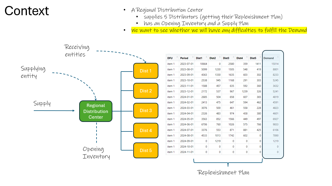
We are going to take as example here the “item 1”.
# get data
data("alloc_data")

# set a working df
df1 <- alloc_data

# filter on the "item1"
df1 <- df1 |> filter(DFU == "item 1")

# keep results
initial_data <- df1

# display
head(df1)
# A tibble: 6 × 10
DFU Period Dist1 Dist2 Dist3 Dist4 Dist5 Demand Opening Supply
<chr> <date> <dbl> <dbl> <dbl> <dbl> <dbl> <dbl> <dbl> <dbl>
1 item 1 2023-07-01 10664 0 2580 359 1411 15014 20000 4000
2 item 1 2023-08-01 5099 1230 1505 548 419 8801 0 1000
3 item 1 2023-09-01 4363 1330 1635 603 302 8233 0 0
4 item 1 2023-10-01 2538 945 1168 291 303 5245 0 17000
5 item 1 2023-11-01 1588 457 635 592 360 3632 0 0
6 item 1 2023-12-01 2172 537 967 1239 326 5241 0 500The variables with each Distributors (Dist1, Dist2,…, Dist5) represent the monthly replenishment plan of each Distributor.
the variable Demand is the sum of those monthly replenishment plan for all the Distributors.
the variable Opening is the Opening stocks at the Supplying entity.
the variable Supply is the Replenishment Plan to the Supplying entity.
39 Calculate Supplier projected inventories
Let’s see whether, considering the total Demand, the Opening Inventories and the current Supply, the projected inventories at the Supplying Entity are :
enough to fulfill all the monthly demands.
or if during some months we foresee that we won’t have enough stocks.
The calculation of the constrained demand will be done using the function const_dmd().
If we don’t have enough stocks, we need to :
identify how much stocks we can have as available.
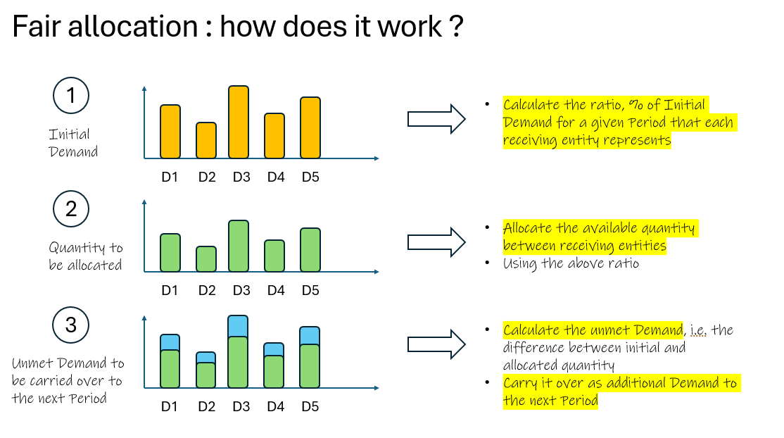
calculate how to do a fair allocation of it between the different Distributors.
This fair allocation will be done considering the % of Demand of each Distributor for a current month.
The calculation of the allocation will be done using the function alloc_dmd().
39.1 Calculate Projected Inventories
First, let’s see whether we have any projected issues : are there some periods of time with not enough stocks to fulfill the Demand ?
For this, we will use the function light_proj_inv() from the R package planr.
39.1.1 Calculation
# set a working df
df1 <- initial_data

# keep only the needed variables
df1 <- df1 |> select(DFU, Period, Demand, Opening, Supply)


# calculate constrained demand
calculated_projection <- planr::light_proj_inv(dataset = df1,
                                          DFU = DFU,
                                          Period = Period,
                                          Demand =  Demand,
                                          Opening = Opening,
                                          Supply = Supply)

glimpse(calculated_projection)
Rows: 17
Columns: 7
$ DFU <chr> "item 1", "item 1", "item 1", "item 1",…
$ Period <date> 2023-07-01, 2023-08-01, 2023-09-01, 20…
$ Demand <dbl> 15014, 8801, 8233, 5245, 3632, 5241, 48…
$ Opening <dbl> 20000, 0, 0, 0, 0, 0, 0, 0, 0, 0, 0, 0,…
$ Calculated.Coverage.in.Periods <dbl> 1.0, 0.1, 0.0, 1.2, 0.2, 0.0, 0.3, 0.4,…
$ Projected.Inventories.Qty <dbl> 8986, 1185, -7048, 4707, 1075, -3666, 1…
$ Supply <dbl> 4000, 1000, 0, 17000, 0, 500, 10000, 50…39.1.2 Display
Let’s look at the results through a nicer table, using the R packages reactable and reactablefmtr :
#-------------------
# Get data
#-------------------

# set a working df
df1 <- calculated_projection


#-------------------
# Transform
#-------------------

# keep only the needed columns
df1 <- df1 |> select(Period,
                      Demand,
                      Calculated.Coverage.in.Periods,
                      Projected.Inventories.Qty,
                      Supply)


# create a f_colorpal field
df1 <- df1 |> mutate(f_colorpal = case_when(
  Calculated.Coverage.in.Periods > 6 ~ "#FFA500",
  Calculated.Coverage.in.Periods > 2 ~ "#32CD32",
  Calculated.Coverage.in.Periods > 0 ~ "#FFFF99",
  TRUE ~ "#FF0000" ))


#-------------------
# Table
#-------------------

# create reactable
reactable(df1, resizable = TRUE, showPageSizeOptions = TRUE,

              striped = TRUE, highlight = TRUE, compact = TRUE,
              defaultPageSize = 20,

              columns = list(

                Demand = colDef(
                  name = "Demand (units)",

                  cell = data_bars(df1,
                                   fill_color = "#3fc1c9",
                                   text_position = "outside-end"
                  )

                ),

              Calculated.Coverage.in.Periods = colDef(
                name = "Coverage (Periods)",
                maxWidth = 90,
                cell= color_tiles(df1, color_ref = "f_colorpal")
              ),

              f_colorpal = colDef(show = FALSE), # hidden, just used for the coverages

                `Projected.Inventories.Qty`= colDef(
                  name = "Projected Inventories (units)",
                  format = colFormat(separators = TRUE, digits=0),

                  style = function(value) {
                    if (value > 0) {
                      color <- "#008000"
                    } else if (value < 0) {
                      color <- "#e00000"
                    } else {
                      color <- "#777"
                    }
                    list(color = color
                    )
                  }
                ),

              Supply = colDef(
                name = "Supply (units)",
                cell = data_bars(df1,
                                 fill_color = "#3CB371",
                                 text_position = "outside-end"
                                 )
                )

              ), # close columns list

              columnGroups = list(

                colGroup(name = "Projected Inventories",
                         columns = c("Calculated.Coverage.in.Periods",
                                     "Projected.Inventories.Qty")
                         )

              )

    ) # close reactable
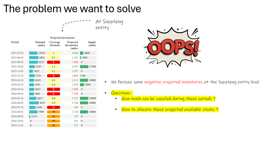
We notice that we have several periods with some negative projected inventories.
Some shortages are even longer than one period, such as March and April 2024, showing 2 consecutive months without enough stocks to fulfill the Demand.
We will need to :
first, calculate the constrained demand, i.e. the quantity which can be supplied during those periods.
and then allocate this available quantity between the receiving entities.
39.2 Calculate Constrained Demand
Now, let’s calculate the constrained demand, using the function const_dmd() from the R packageplanr.
# set a working df
df1 <- initial_data

# keep only the needed variables
df1 <- df1 |> select(DFU, Period, Demand, Opening, Supply)


# calculate constrained demand
calculated_projection <- planr::const_dmd(dataset = df1,
                                          DFU = DFU,
                                          Period = Period,
                                          Demand =  Demand,
                                          Opening = Opening,
                                          Supply = Supply)


glimpse(calculated_projection)
Rows: 17
Columns: 9
$ DFU <chr> "item 1", "item 1", "item 1", "item 1",…
$ Period <date> 2023-07-01, 2023-08-01, 2023-09-01, 20…
$ Demand <dbl> 15014, 8801, 8233, 5245, 3632, 5241, 48…
$ Opening <dbl> 20000, 0, 0, 0, 0, 0, 0, 0, 0, 0, 0, 0,…
$ Calculated.Coverage.in.Periods <dbl> 1.0, 0.1, 0.0, 1.2, 0.2, 0.0, 0.3, 0.4,…
$ Projected.Inventories.Qty <dbl> 8986, 1185, -7048, 4707, 1075, -3666, 1…
$ Supply <dbl> 4000, 1000, 0, 17000, 0, 500, 10000, 50…
$ Constrained.Demand <dbl> 15014, 8801, 1185, 12293, 3632, 1575, 8…
$ Current.Stock.Available.Tag <dbl> 1, 0, 0, 0, 0, 0, 0, 0, 0, 0, 0, 0, 0, …39.3 Displays
Let’s create 2 nicer displays.
39.3.1 At Supplier level
We create first a function status_badge that we will use to display in the reactable :
#---------------------------------------------------------
#    A Function to define a Badge Status in the reactable
#---------------------------------------------------------

status_badge <- function(color = "#aaa", width = "9px", height = width) {
  span(style = list(
    display = "inline-block",
    marginRight = "8px",
    width = width,
    height = height,
    backgroundColor = color,
    borderRadius = "50%"
  ))
}
Now we create the reactable :
# set a working df
df1 <- calculated_projection


#----------------
# Create the table
#----------------

# remove not needed column
df1 <- df1 |> select(-DFU)

# reorder variables
df1 <- df1 |> select(Period, Demand, Constrained.Demand,
                     Current.Stock.Available.Tag,
                     Calculated.Coverage.in.Periods,
                     Projected.Inventories.Qty, Supply
                     )

# create a f_colorpal field
df1 <- df1 |> mutate(f_colorpal = case_when(
  Calculated.Coverage.in.Periods > 6 ~ "#FFA500",
  Calculated.Coverage.in.Periods > 2 ~ "#32CD32",
  Calculated.Coverage.in.Periods > 0 ~ "#FFFF99",
  TRUE ~ "#FF0000" ))


# adjust Current.Stock.Available.Tag
df1$Current.Stock.Available.Tag <- if_else(df1$Current.Stock.Available.Tag == 1, "Available", "")


#-------------------------
# Create Table

reactable(df1, resizable = TRUE, showPageSizeOptions = TRUE,

              striped = TRUE, highlight = TRUE, compact = TRUE,
              defaultPageSize = 20,

              columns = list(


                Demand = colDef(
                  name = "Demand (units)",

                  cell = data_bars(df1,
                                   fill_color = "#3fc1c9",
                                   text_position = "outside-end")

                ),

                Constrained.Demand = colDef(

                  name = "Constrained Demand (units)",

                  cell = data_bars(df1,
                                   fill_color = "gold",
                                   text_position = "outside-end")

                ),


                Calculated.Coverage.in.Periods = colDef(
                  name = "Coverage (Periods)",
                  maxWidth = 90,

                  cell= color_tiles(df1, color_ref = "f_colorpal")
                ),


                f_colorpal = colDef(show = FALSE), # hidden, just used for the coverages


                `Projected.Inventories.Qty`= colDef(
                  name = "Projected Inventories (units)",
                  format = colFormat(separators = TRUE, digits=0),

                  style = function(value) {
                    if (value > 0) {
                      color <- "#008000"
                    } else if (value < 0) {
                      color <- "#e00000"
                    } else {
                      color <- "#777"
                    }
                    list(color = color
                    )
                  }
                ),


                Current.Stock.Available.Tag = colDef(
                  name = "Current Stock Available Tag",

                  cell = function(value) {
                    color <- switch(
                      value,
                      No = "hsl(120,61%,50%)",
                      Available = "rgb(135,206,250)"
                    )
                    badge <- status_badge(color = color)
                    tagList(badge, value)
                  }),


                Supply = colDef(
                  name = "Supply (units)",
                  cell = data_bars(df1,
                                   fill_color = "#3CB371",
                                   text_position = "outside-end"
                  )
                )


              ), # close columns list

              columnGroups = list(

                colGroup(name = "Projected Inventories",
                         columns = c("Calculated.Coverage.in.Periods",
                                     "Projected.Inventories.Qty")
                         )

              )

    ) # close reactable
We can see that several periods have some negative projected inventories :
the projected available demand at those moments will need to be allocated to the different distributors.
the unmet demand will need to be carried over to the next period of time.
The function alloc_dmd() will perform all those 4 operations :
calculate the constrained demand.
identify the periods of time where an allocation is needed.
allocate the available constrained demand at those periods.
carry over to the next period of time the unmet demand, by receiving entities.
39.3.2 Including Distributors demand
If we want more details about the Demand, we also can display the Demand of all the Distributors, as illustrated in the following table.
#-------------------------
# Get detailed demand of each Distributor
#-------------------------

# set a working df
df1 <- initial_data

# keep only needed variables
df1 <- df1 |> select(-Demand,
                     -Opening,
                     -Supply)

#-------------------------
# Combine w/ calculated_projection
#-------------------------

# merge
df1 <- left_join(df1, calculated_projection)


#-------------------------
# Create table
#-------------------------

# remove not needed column
df1 <- df1 |> select(-DFU)


# reorder variables
df1 <- df1 |> select(Period,

                     # details of the Demand
                     Dist1,
                     Dist2,
                     Dist3,
                     Dist4,
                     Dist5,
                     Demand,

                     Constrained.Demand,
                     Current.Stock.Available.Tag,
                     Calculated.Coverage.in.Periods,
                     Projected.Inventories.Qty, Supply
                     )

# create a f_colorpal field
df1 <- df1 |> mutate(f_colorpal = case_when(
  Calculated.Coverage.in.Periods > 6 ~ "#FFA500",
  Calculated.Coverage.in.Periods > 2 ~ "#32CD32",
  Calculated.Coverage.in.Periods > 0 ~ "#FFFF99",
  TRUE ~ "#FF0000" ))


# adjust Current.Stock.Available.Tag
df1$Current.Stock.Available.Tag <- if_else(df1$Current.Stock.Available.Tag == 1, "Available", "")


#-------------------------
# Create Table

reactable(df1, resizable = TRUE, showPageSizeOptions = TRUE,

              striped = TRUE, highlight = TRUE, compact = TRUE,
              defaultPageSize = 20,

              columns = list(

                Period = colDef(name = "Period",
                                sticky = "left"
                                ),


                #-----------------------
                # Details demand

                `Dist1`= colDef(
                  name = "Dist1 (units)",
                  format = colFormat(separators = TRUE, digits=0)
                  ),

                `Dist2`= colDef(
                  name = "Dist2 (units)",
                  format = colFormat(separators = TRUE, digits=0)
                  ),

                `Dist3`= colDef(
                  name = "Dist3 (units)",
                  format = colFormat(separators = TRUE, digits=0)
                  ),

                `Dist4`= colDef(
                  name = "Dist4 (units)",
                  format = colFormat(separators = TRUE, digits=0)
                  ),

                `Dist5`= colDef(
                  name = "Dist5 (units)",
                  format = colFormat(separators = TRUE, digits=0)
                  ),


                Demand = colDef(
                  name = "Total Demand (units)",

                  cell = data_bars(df1,
                                   fill_color = "#3fc1c9",
                                   text_position = "outside-end")

                ),

                Constrained.Demand = colDef(

                  name = "Constrained Demand (units)",

                  cell = data_bars(df1,
                                   fill_color = "gold",
                                   text_position = "outside-end")

                ),


                Calculated.Coverage.in.Periods = colDef(
                  name = "Coverage (Periods)",
                  maxWidth = 90,

                  cell= color_tiles(df1, color_ref = "f_colorpal")
                ),


                f_colorpal = colDef(show = FALSE), # hidden, just used for the coverages


                `Projected.Inventories.Qty`= colDef(
                  name = "Projected Inventories (units)",
                  format = colFormat(separators = TRUE, digits=0),

                  style = function(value) {
                    if (value > 0) {
                      color <- "#008000"
                    } else if (value < 0) {
                      color <- "#e00000"
                    } else {
                      color <- "#777"
                    }
                    list(color = color
                    )
                  }
                ),


                Current.Stock.Available.Tag = colDef(
                  name = "Current Stock Available Tag",

                  cell = function(value) {
                    color <- switch(
                      value,
                      No = "hsl(120,61%,50%)",
                      Available = "rgb(135,206,250)"
                    )
                    badge <- status_badge(color = color)
                    tagList(badge, value)
                  }),


                Supply = colDef(
                  name = "Supply (units)",
                  cell = data_bars(df1,
                                   fill_color = "#3CB371",
                                   text_position = "outside-end"
                  )
                )


              ), # close columns list

              columnGroups = list(


                colGroup(name = "Details Demand",
                         columns = c("Dist1",
                                     "Dist2",
                                     "Dist3",
                                     "Dist4",
                                     "Dist5")),


                colGroup(name = "Projected Inventories",
                         columns = c("Calculated.Coverage.in.Periods",
                                     "Projected.Inventories.Qty"))

              )

    ) # close reactable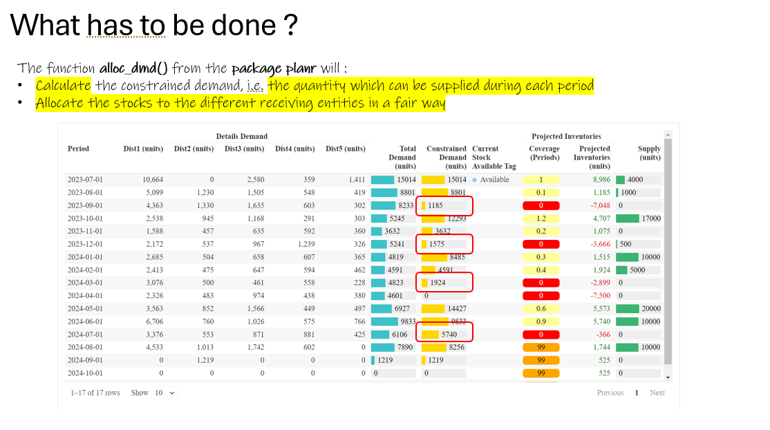
As we can see, we have 2 consecutive periods of time with negative projected inventories : March 2024 and April 2024.
Therefore, we will need to proceed with “2 rounds” of allocation of demand.
40 Allocate Demand | Round 1
We proceed in 2 steps :
Step 1 : allocate the Demand, using the function
alloc_dmd().Step 2 : get the new Constrained Demand, using the function
const_dmd().
40.1 Calculations
40.1.1 Step 1 : Allocate Demand
# calculate allocated demand
allocated_demand_data <- alloc_dmd(dataset = initial_data,
                 DFU = DFU,
                 Period = Period,
                 Demand = Demand,
                 Opening = Opening,
                 Supply = Supply)

glimpse(allocated_demand_data)
Rows: 17
Columns: 10
$ DFU <chr> "item 1", "item 1", "item 1", "item 1", "item 1", "item 1", "i…
$ Period <date> 2023-07-01, 2023-08-01, 2023-09-01, 2023-10-01, 2023-11-01, 2…
$ Dist1 <dbl> 10664.0000, 5099.0000, 627.9795, 6273.0205, 1588.0000, 652.718…
$ Dist2 <dbl> 0.0000, 1230.0000, 191.4308, 2083.5692, 457.0000, 161.3766, 87…
$ Dist3 <dbl> 2580.0000, 1505.0000, 235.3304, 2567.6696, 635.0000, 290.5982,…
$ Dist4 <dbl> 359.00000, 548.00000, 86.79157, 807.20843, 592.00000, 372.3382…
$ Dist5 <dbl> 1411.00000, 419.00000, 43.46775, 561.53225, 360.00000, 97.9679…
$ Demand <dbl> 15014, 8801, 1185, 12293, 3632, 1575, 8485, 4591, 1924, 7500, …
$ Opening <dbl> 20000, 0, 0, 0, 0, 0, 0, 0, 0, 0, 0, 0, 0, 0, 0, 0, 0
$ Supply <dbl> 4000, 1000, 0, 17000, 0, 500, 10000, 5000, 0, 0, 20000, 10000,…We can see that :
the constrained demand identified on the initial dataset now became the new Demand.
the related demand of each distributor during this period of time has also been allocated to match with this new Demand.
40.1.2 Step 2 : Get New Constrained Demand
# set a working df
df1 <- allocated_demand_data

# keep only the needed variables
df1 <- df1 |> select(DFU, Period, Demand, Opening, Supply)


# calculate constrained demand
new_calculated_projection <- planr::const_dmd(dataset = df1,
                                          DFU = DFU,
                                          Period = Period,
                                          Demand =  Demand,
                                          Opening = Opening,
                                          Supply = Supply)


glimpse(new_calculated_projection)
Rows: 17
Columns: 9
$ DFU <chr> "item 1", "item 1", "item 1", "item 1",…
$ Period <date> 2023-07-01, 2023-08-01, 2023-09-01, 20…
$ Demand <dbl> 15014, 8801, 1185, 12293, 3632, 1575, 8…
$ Opening <dbl> 20000, 0, 0, 0, 0, 0, 0, 0, 0, 0, 0, 0,…
$ Calculated.Coverage.in.Periods <dbl> 1.2, 1.0, 0.0, 1.7, 0.7, 0.0, 0.3, 1.0,…
$ Projected.Inventories.Qty <dbl> 8986, 1185, 0, 4707, 1075, 0, 1515, 192…
$ Supply <dbl> 4000, 1000, 0, 17000, 0, 500, 10000, 50…
$ Constrained.Demand <dbl> 15014, 8801, 1185, 12293, 3632, 1575, 8…
$ Current.Stock.Available.Tag <dbl> 1, 0, 0, 0, 0, 0, 0, 0, 0, 0, 0, 0, 0, …Now we can see that the projected inventories are equal to zero for each first period when an allocation was needed.
The only exception is the month of April 2024.
This month was a consecutive month with negative projected inventories.
A second round of allocation is then needed to allocate the demand of this month.
Let’s note that the Constrained Demand is equal to zero, which means :
there won’t be any available stocks to allocate.
the missing quantity (here 7500 units) will need to be carried over the next period of time.
40.2 Display
Let’s look at the tables through nicer visuals :
40.2.1 At Supplier level
# set a working df
df1 <- new_calculated_projection


#----------------
# Create the table
#----------------

# remove not needed column
df1 <- df1 |> select(-DFU)


# reorder variables
df1 <- df1 |> select(Period, Demand, Constrained.Demand,
                     Current.Stock.Available.Tag,
                     Calculated.Coverage.in.Periods,
                     Projected.Inventories.Qty, Supply
                     )

# create a f_colorpal field
df1 <- df1 |> mutate(f_colorpal = case_when(
  Calculated.Coverage.in.Periods > 6 ~ "#FFA500",
  Calculated.Coverage.in.Periods > 2 ~ "#32CD32",
  Calculated.Coverage.in.Periods > 0 ~ "#FFFF99",
  TRUE ~ "#FF0000" ))


# adjust Current.Stock.Available.Tag
df1$Current.Stock.Available.Tag <- if_else(df1$Current.Stock.Available.Tag == 1, "Available", "")


#-------------------------
# Create Table

reactable(df1, resizable = TRUE, showPageSizeOptions = TRUE,

              striped = TRUE, highlight = TRUE, compact = TRUE,
              defaultPageSize = 20,

              columns = list(


                Demand = colDef(
                  name = "Demand (units)",

                  cell = data_bars(df1,
                                   fill_color = "#3fc1c9",
                                   text_position = "outside-end")

                ),

                Constrained.Demand = colDef(

                  name = "Constrained Demand (units)",

                  cell = data_bars(df1,
                                   fill_color = "gold",
                                   text_position = "outside-end")

                ),


                Calculated.Coverage.in.Periods = colDef(
                  name = "Coverage (Periods)",
                  maxWidth = 90,

                  cell= color_tiles(df1, color_ref = "f_colorpal")
                ),


                f_colorpal = colDef(show = FALSE), # hidden, just used for the coverages


                `Projected.Inventories.Qty`= colDef(
                  name = "Projected Inventories (units)",
                  format = colFormat(separators = TRUE, digits=0),

                  style = function(value) {
                    if (value > 0) {
                      color <- "#008000"
                    } else if (value < 0) {
                      color <- "#e00000"
                    } else {
                      color <- "#777"
                    }
                    list(color = color
                    )
                  }
                ),


                Current.Stock.Available.Tag = colDef(
                  name = "Current Stock Available Tag",

                  cell = function(value) {
                    color <- switch(
                      value,
                      No = "hsl(120,61%,50%)",
                      Available = "rgb(135,206,250)"
                    )
                    badge <- status_badge(color = color)
                    tagList(badge, value)
                  }),


                Supply = colDef(
                  name = "Supply (units)",
                  cell = data_bars(df1,
                                   fill_color = "#3CB371",
                                   text_position = "outside-end"
                  )
                )


              ), # close columns list

              columnGroups = list(

                colGroup(name = "Projected Inventories",
                         columns = c("Calculated.Coverage.in.Periods",
                                     "Projected.Inventories.Qty")
                         )

              )

    ) # close reactable
For the previous period of time where we were in shortages, now :
the Constrained Demand is equal to the Demand.
the projected inventories are equal to zero.
There is still one period of time where another round of allocation is needed : April 2024.
Now let’s look at the new allocated demand by distributors.
40.2.2 Including Distributors new demand
#-------------------------
# Get detailed new demand of each Distributor
#-------------------------

# set a working df
df1 <- allocated_demand_data

# keep only needed variables
df1 <- df1 |> select(-Demand,
                     -Opening,
                     -Supply)

#-------------------------
# Combine w/ new_calculated_projection
#-------------------------

# merge
df1 <- left_join(df1, new_calculated_projection)


#-------------------------
# Create table
#-------------------------

# remove not needed column
df1 <- df1 |> select(-DFU)

# reorder variables
df1 <- df1 |> select(Period,

                     # details of the Demand
                     Dist1,
                     Dist2,
                     Dist3,
                     Dist4,
                     Dist5,
                     Demand,

                     Constrained.Demand,
                     Current.Stock.Available.Tag,
                     Calculated.Coverage.in.Periods,
                     Projected.Inventories.Qty, Supply
                     )

# create a f_colorpal field
df1 <- df1 |> mutate(f_colorpal = case_when(
  Calculated.Coverage.in.Periods > 6 ~ "#FFA500",
  Calculated.Coverage.in.Periods > 2 ~ "#32CD32",
  Calculated.Coverage.in.Periods > 0 ~ "#FFFF99",
  TRUE ~ "#FF0000" ))


# adjust Current.Stock.Available.Tag
df1$Current.Stock.Available.Tag <- if_else(df1$Current.Stock.Available.Tag == 1, "Available", "")


#-------------------------
# Create Table

reactable(df1, resizable = TRUE, showPageSizeOptions = TRUE,

              striped = TRUE, highlight = TRUE, compact = TRUE,
              defaultPageSize = 20,

              columns = list(

                Period = colDef(name = "Period",
                                sticky = "left"
                                ),


                #-----------------------
                # Details demand

                `Dist1`= colDef(
                  name = "Dist1 (units)",
                  format = colFormat(separators = TRUE, digits=0)
                  ),

                `Dist2`= colDef(
                  name = "Dist2 (units)",
                  format = colFormat(separators = TRUE, digits=0)
                  ),

                `Dist3`= colDef(
                  name = "Dist3 (units)",
                  format = colFormat(separators = TRUE, digits=0)
                  ),

                `Dist4`= colDef(
                  name = "Dist4 (units)",
                  format = colFormat(separators = TRUE, digits=0)
                  ),

                `Dist5`= colDef(
                  name = "Dist5 (units)",
                  format = colFormat(separators = TRUE, digits=0)
                  ),


                Demand = colDef(
                  name = "Total Demand (units)",

                  cell = data_bars(df1,
                                   fill_color = "#3fc1c9",
                                   text_position = "outside-end")

                ),


                Calculated.Coverage.in.Periods = colDef(
                  name = "Coverage (Periods)",
                  maxWidth = 90,

                  cell= color_tiles(df1, color_ref = "f_colorpal")
                ),


                f_colorpal = colDef(show = FALSE), # hidden, just used for the coverages


                `Projected.Inventories.Qty`= colDef(
                  name = "Projected Inventories (units)",
                  format = colFormat(separators = TRUE, digits=0),

                  style = function(value) {
                    if (value > 0) {
                      color <- "#008000"
                    } else if (value < 0) {
                      color <- "#e00000"
                    } else {
                      color <- "#777"
                    }
                    list(color = color
                    )
                  }
                ),


                Supply = colDef(
                  name = "Supply (units)",
                  cell = data_bars(df1,
                                   fill_color = "#3CB371",
                                   text_position = "outside-end"
                  )
                )


              ), # close columns lits

              columnGroups = list(


                colGroup(name = "Details Demand",
                         columns = c("Dist1",
                                     "Dist2",
                                     "Dist3",
                                     "Dist4",
                                     "Dist5")),


                colGroup(name = "Projected Inventories",
                         columns = c("Calculated.Coverage.in.Periods",
                                     "Projected.Inventories.Qty"))

              )

    ) # close reactable
41 Allocate Demand | Round 2
41.1 Prepare template
It’s simply the new template calculated after the first round of allocation.
# Get new template
# with detailed new demand of each Distributor
round1_data <- allocated_demand_data

glimpse(df1)
Rows: 17
Columns: 13
$ Period <date> 2023-07-01, 2023-08-01, 2023-09-01, 20…
$ Dist1 <dbl> 10664.0000, 5099.0000, 627.9795, 6273.0…
$ Dist2 <dbl> 0.0000, 1230.0000, 191.4308, 2083.5692,…
$ Dist3 <dbl> 2580.0000, 1505.0000, 235.3304, 2567.66…
$ Dist4 <dbl> 359.00000, 548.00000, 86.79157, 807.208…
$ Dist5 <dbl> 1411.00000, 419.00000, 43.46775, 561.53…
$ Demand <dbl> 15014, 8801, 1185, 12293, 3632, 1575, 8…
$ Constrained.Demand <dbl> 15014, 8801, 1185, 12293, 3632, 1575, 8…
$ Current.Stock.Available.Tag <chr> "Available", "", "", "", "", "", "", ""…
$ Calculated.Coverage.in.Periods <dbl> 1.2, 1.0, 0.0, 1.7, 0.7, 0.0, 0.3, 1.0,…
$ Projected.Inventories.Qty <dbl> 8986, 1185, 0, 4707, 1075, 0, 1515, 192…
$ Supply <dbl> 4000, 1000, 0, 17000, 0, 500, 10000, 50…
$ f_colorpal <chr> "#FFFF99", "#FFFF99", "#FF0000", "#FFFF…41.2 Calculations
We repeat the same steps that we did before.
41.2.1 Step 1 : Allocate Demand
# calculate allocated demand
allocated_demand_data <- alloc_dmd(dataset = round1_data,
                 DFU = DFU,
                 Period = Period,
                 Demand = Demand,
                 Opening = Opening,
                 Supply = Supply)

glimpse(allocated_demand_data)
Rows: 17
Columns: 10
$ DFU <chr> "item 1", "item 1", "item 1", "item 1", "item 1", "item 1", "i…
$ Period <date> 2023-07-01, 2023-08-01, 2023-09-01, 2023-10-01, 2023-11-01, 2…
$ Dist1 <dbl> 10664.0000, 5099.0000, 627.9795, 6273.0205, 1588.0000, 652.718…
$ Dist2 <dbl> 0.0000, 1230.0000, 191.4308, 2083.5692, 457.0000, 161.3766, 87…
$ Dist3 <dbl> 2580.0000, 1505.0000, 235.3304, 2567.6696, 635.0000, 290.5982,…
$ Dist4 <dbl> 359.00000, 548.00000, 86.79157, 807.20843, 592.00000, 372.3382…
$ Dist5 <dbl> 1411.00000, 419.00000, 43.46775, 561.53225, 360.00000, 97.9679…
$ Demand <dbl> 15014, 8801, 1185, 12293, 3632, 1575, 8485, 4591, 1924, 0, 144…
$ Opening <dbl> 20000, 0, 0, 0, 0, 0, 0, 0, 0, 0, 0, 0, 0, 0, 0, 0, 0
$ Supply <dbl> 4000, 1000, 0, 17000, 0, 500, 10000, 5000, 0, 0, 20000, 10000,…41.2.2 Step 2 : Get New Constrained Demand
# set a working df
df1 <- allocated_demand_data

# keep only the needed variables
df1 <- df1 |> select(DFU, Period, Demand, Opening, Supply)


# calculate constrained demand
new_calculated_projection <- planr::const_dmd(dataset = df1,
                                          DFU = DFU,
                                          Period = Period,
                                          Demand =  Demand,
                                          Opening = Opening,
                                          Supply = Supply)


glimpse(new_calculated_projection)
Rows: 17
Columns: 9
$ DFU <chr> "item 1", "item 1", "item 1", "item 1",…
$ Period <date> 2023-07-01, 2023-08-01, 2023-09-01, 20…
$ Demand <dbl> 15014, 8801, 1185, 12293, 3632, 1575, 8…
$ Opening <dbl> 20000, 0, 0, 0, 0, 0, 0, 0, 0, 0, 0, 0,…
$ Calculated.Coverage.in.Periods <dbl> 1.2, 1.0, 0.0, 1.7, 0.7, 0.0, 0.3, 1.0,…
$ Projected.Inventories.Qty <dbl> 8986, 1185, 0, 4707, 1075, 0, 1515, 192…
$ Supply <dbl> 4000, 1000, 0, 17000, 0, 500, 10000, 50…
$ Constrained.Demand <dbl> 15014, 8801, 1185, 12293, 3632, 1575, 8…
$ Current.Stock.Available.Tag <dbl> 1, 0, 0, 0, 0, 0, 0, 0, 0, 0, 0, 0, 0, …41.3 Display
41.3.1 At Supplier level
# set a working df
df1 <- new_calculated_projection


#----------------
# Create the table
#----------------

# remove not needed column
df1 <- df1 |> select(-DFU)


# reorder variables
df1 <- df1 |> select(Period,
                     Demand,
                     Constrained.Demand,
                     Current.Stock.Available.Tag,
                     Calculated.Coverage.in.Periods,
                     Projected.Inventories.Qty, Supply
                     )

# create a f_colorpal field
df1 <- df1 |> mutate(f_colorpal = case_when(
  Calculated.Coverage.in.Periods > 6 ~ "#FFA500",
  Calculated.Coverage.in.Periods > 2 ~ "#32CD32",
  Calculated.Coverage.in.Periods > 0 ~ "#FFFF99",
  TRUE ~ "#FF0000" ))


# adjust Current.Stock.Available.Tag
df1$Current.Stock.Available.Tag <- if_else(df1$Current.Stock.Available.Tag == 1, "Available", "")


#-------------------------
# Create Table

reactable(df1, resizable = TRUE, showPageSizeOptions = TRUE,

              striped = TRUE, highlight = TRUE, compact = TRUE,
              defaultPageSize = 20,

              columns = list(


                Demand = colDef(
                  name = "Demand (units)",

                  cell = data_bars(df1,
                                   fill_color = "#3fc1c9",
                                   text_position = "outside-end")

                ),

                Constrained.Demand = colDef(

                  name = "Constrained Demand (units)",

                  cell = data_bars(df1,
                                   fill_color = "gold",
                                   text_position = "outside-end")

                ),


                Calculated.Coverage.in.Periods = colDef(
                  name = "Coverage (Periods)",
                  maxWidth = 90,

                  cell= color_tiles(df1, color_ref = "f_colorpal")
                ),


                f_colorpal = colDef(show = FALSE), # hidden, just used for the coverages


                `Projected.Inventories.Qty`= colDef(
                  name = "Projected Inventories (units)",
                  format = colFormat(separators = TRUE, digits=0),

                  style = function(value) {
                    if (value > 0) {
                      color <- "#008000"
                    } else if (value < 0) {
                      color <- "#e00000"
                    } else {
                      color <- "#777"
                    }
                    list(color = color
                         #fontWeight = "bold"
                    )
                  }
                ),


                Current.Stock.Available.Tag = colDef(
                  name = "Current Stock Available Tag",

                  cell = function(value) {
                    color <- switch(
                      value,
                      No = "hsl(120,61%,50%)",
                      Available = "rgb(135,206,250)"
                    )
                    badge <- status_badge(color = color)
                    tagList(badge, value)
                  }),


                Supply = colDef(
                  name = "Supply (units)",
                  cell = data_bars(df1,
                                   fill_color = "#3CB371",
                                   text_position = "outside-end"
                  )
                )


              ), # close columns list

              columnGroups = list(
                colGroup(name = "Projected Inventories",
                         columns = c("Calculated.Coverage.in.Periods",
                                     "Projected.Inventories.Qty"))

              )

    ) # close reactable
41.3.2 Including Distributors new demand
#-------------------------
# Get detailed new demand of each Distributor
#-------------------------

# set a working df
df1 <- allocated_demand_data

# keep only needed variables
df1 <- df1 |> select(-Demand,
                     -Opening,
                     -Supply)

#-------------------------
# Combine w/ new_calculated_projection
#-------------------------

# merge
df1 <- left_join(df1, new_calculated_projection)


#-------------------------
# Create table
#-------------------------

# remove not needed column
df1 <- df1 |> select(-DFU)


# reorder variables
df1 <- df1 |> select(Period,

                     # details of the Demand
                     Dist1,
                     Dist2,
                     Dist3,
                     Dist4,
                     Dist5,
                     Demand,

                     Constrained.Demand,
                     Current.Stock.Available.Tag,
                     Calculated.Coverage.in.Periods,
                     Projected.Inventories.Qty,
                     Supply
                     )

# create a f_colorpal field
df1 <- df1 |> mutate(f_colorpal = case_when(
  Calculated.Coverage.in.Periods > 6 ~ "#FFA500",
  Calculated.Coverage.in.Periods > 2 ~ "#32CD32",
  Calculated.Coverage.in.Periods > 0 ~ "#FFFF99",
  TRUE ~ "#FF0000" ))


# adjust Current.Stock.Available.Tag
df1$Current.Stock.Available.Tag <- if_else(df1$Current.Stock.Available.Tag == 1, "Available", "")


#-------------------------
# Create Table

reactable(df1, resizable = TRUE, showPageSizeOptions = TRUE,

              striped = TRUE, highlight = TRUE, compact = TRUE,
              defaultPageSize = 20,

              columns = list(

                Period = colDef(name = "Period",
                                sticky = "left"
                                ),


                #-----------------------
                # Details demand

                `Dist1`= colDef(
                  name = "Dist1 (units)",
                  format = colFormat(separators = TRUE, digits=0)
                  ),

                `Dist2`= colDef(
                  name = "Dist2 (units)",
                  format = colFormat(separators = TRUE, digits=0)
                  ),

                `Dist3`= colDef(
                  name = "Dist3 (units)",
                  format = colFormat(separators = TRUE, digits=0)
                  ),

                `Dist4`= colDef(
                  name = "Dist4 (units)",
                  format = colFormat(separators = TRUE, digits=0)
                  ),

                `Dist5`= colDef(
                  name = "Dist5 (units)",
                  format = colFormat(separators = TRUE, digits=0)
                  ),


                Demand = colDef(
                  name = "Total Demand (units)",

                  cell = data_bars(df1,
                                   fill_color = "#3fc1c9",
                                   text_position = "outside-end")

                ),


                Calculated.Coverage.in.Periods = colDef(
                  name = "Coverage (Periods)",
                  maxWidth = 90,

                  cell= color_tiles(df1, color_ref = "f_colorpal")
                ),


                f_colorpal = colDef(show = FALSE), # hidden, just used for the coverages


                `Projected.Inventories.Qty`= colDef(
                  name = "Projected Inventories (units)",
                  format = colFormat(separators = TRUE, digits=0),

                  style = function(value) {
                    if (value > 0) {
                      color <- "#008000"
                    } else if (value < 0) {
                      color <- "#e00000"
                    } else {
                      color <- "#777"
                    }
                    list(color = color
                    )
                  }
                ),


                Supply = colDef(
                  name = "Supply (units)",
                  cell = data_bars(df1,
                                   fill_color = "#3CB371",
                                   text_position = "outside-end"
                  )
                )


              ), # close columns list

              columnGroups = list(


                colGroup(name = "Details Demand",
                         columns = c("Dist1",
                                     "Dist2",
                                     "Dist3",
                                     "Dist4",
                                     "Dist5")),


                colGroup(name = "Projected Inventories",
                         columns = c("Calculated.Coverage.in.Periods",
                                     "Projected.Inventories.Qty"))

              )

    ) # close reactable
42 Finaly : Check totals
Let’s check the total of the new allocated demand of each distributors, and compare it with the initial demand (not allocated).
We can write (in an excel or csv file) the 2 data frames to compare them.
We can see that for each Distributor the total Demand is the same over the full horizon : the monthly Demand has been allocated considering the supply availability.
# initial dataset
#write.csv(initial_data, file = "initial_data.csv")


# allocated_demand_data
#write.csv(allocated_demand_data, file = "allocated_demand_data.csv")